Sys.setenv(POLARS_MAX_THREADS = as.character(params$threads))Working with large data in R
data.table, Arrow, DuckDB and Polars: what each is good at, and when to reach for it
1 Introduction
There is a size of dataset, somewhere between “opens in Excel” and “needs a cluster”, where the tool you choose matters more than the code you write with it. A table of a few tens of millions of rows fits on a laptop’s disk comfortably and in its memory uncomfortably, and the difference between a good and bad choice of library is not ten percent. As we will see, it is closer to a factor of a hundred.
This workshop works through six realistic genomics workflows on a 46-million-row variant table and a 20,000 × 2,778 expression matrix, using the main options available in R today: base R, dplyr, data.table, collapse, GenomicRanges, Arrow, DuckDB and Polars. For each we measure how long it takes and how much memory it needs, verify that every implementation produces the same answer, and, more usefully than either, work out what each tool is actually for.
| Workflow | Shape | What it tests | |
|---|---|---|---|
| 1 | Subclonal mutation fraction | Grouped aggregation | The baseline case: 46M rows in, 2,778 out |
| 2 | Variant → gene assignment | Range join | Where specialized interval tools match the column stores |
| 3 | Mutation density in bins | High-cardinality group-by | The cost of a large result |
| 4 | Flagging known variants | Large-to-large equi-join | The case that exhausts memory |
| 5 | RNAseq QC and normalization | Matrix algebra | Where relational engines stop being the answer |
| 6 | sMF versus expression | All of the above | Global normalization feeding a narrow question |
The short version, if you want to stop reading after one paragraph: store your data as Parquet, and use an engine that can query it without loading it. Workflows 1, 3, 4 and 6 are the evidence for that sentence; workflows 2 and 5 are the honest qualifications to it.
TipRunning this document
The params: block at the top of the source controls cost:
scale: "demo"builds a 200-sample subset and renders in a few minutes. Use it while you are editing.run_read_table: falseskips the single slowest chunk.threadscaps every engine to the same number of cores. Comparing 16-thread DuckDB against single-threaded base R is not a benchmark, it is a press release.
2 Setup
ImportantThread caps must come first
POLARS_MAX_THREADS is read when Polars’ Rust thread pool initializes and cannot be changed after library(polars). It has to be set before the package is loaded, so this is the first executable line in the document.
suppressPackageStartupMessages({
  library(dplyr);  library(ggplot2); library(data.table); library(collapse)
  library(arrow);  library(DBI);     library(duckdb)
  library(duckplyr, warn.conflicts = FALSE)
  library(polars); library(tidypolars)
  library(knitr)
})
source("bench_helpers.R")   # measurement utilities -- see @sec-bench

data.table::setDTthreads(params$threads)
arrow::set_cpu_count(params$threads)

theme_set(theme_minimal(base_size = 12) +
          theme(legend.position = "none",
                panel.grid.minor = element_blank(),
                plot.title.position = "plot"))
fam_pal <- c("base R" = "#7B6B8F", "tidyverse" = "#4C6EA8", "data.table" = "#3E8E7E",
             "collapse" = "#6AA84F", "arrow" = "#C0873F", "polars" = "#B4534B",
             "DuckDB" = "#2F6D8C", "other" = "#8A8A8A")
Machine and package versions
hw <- hardware_info()
tibble::tibble(
  Item  = c("OS", "R", "CPU (logical / physical)", "RAM", "Thread cap"),
  Value = c(hw$os, hw$r_version, paste(hw$logical_cpu, "/", hw$phys_cpu),
            sprintf("%.1f GB", hw$ram_gb), as.character(params$threads))
) |> kable()| Item | Value |
|---|---|
| OS | Windows 10 x64 |
| R | 4.5.1 |
| CPU (logical / physical) | 16 / 8 |
| RAM | 93.6 GB |
| Thread cap | 8 |
Machine and package versions
pkgs <- c("polars", "tidypolars", "duckdb", "duckplyr", "arrow",
          "data.table", "dplyr", "collapse", "fst", "qs2")
tibble::tibble(Package = pkgs, Version = vapply(pkgs, pkg_ver, character(1))) |>
kable(caption = "Package versions used for these results")| Package | Version |
|---|---|
| polars | 1.13.0 |
| tidypolars | 0.19.0 |
| duckdb | 1.5.5 |
| duckplyr | 1.2.1 |
| arrow | 25.0.0 |
| data.table | 1.17.8 |
| dplyr | 1.2.0 |
| collapse | 2.1.7 |
| fst | 0.9.8 |
| qs2 | 0.2.2 |
2.1 The dataset
The example is aggregated CliPP output for all PCAWG samples. To avoid any issues with protected data, the file below has the same shape as real CliPP output, with the same row count, sample count and columns, but the values are randomly generated.
FULL_TSV <- "fake_pcawg_all.tsv"
FULL_PQ  <- "fake_pcawg_all.parquet"

con0 <- dbConnect(duckdb())
if (identical(params$scale, "demo")) {
  PQ <- "dev_subsample.parquet"
  if (!file.exists(PQ)) {
    dbExecute(con0, sprintf("
      COPY (SELECT * FROM read_parquet('%s') WHERE samplename IN (
              SELECT samplename FROM read_parquet('%s')
              GROUP BY samplename ORDER BY samplename LIMIT 200))
      TO '%s' (FORMAT PARQUET, COMPRESSION ZSTD)", FULL_PQ, FULL_PQ, PQ))
  }
  TSV <- NA_character_
  DB  <- "dev_subsample.duckdb"
  if (!file.exists(DB)) {
    cdb <- dbConnect(duckdb(), DB)
    dbExecute(cdb, sprintf("CREATE TABLE pcawg_all AS SELECT * FROM read_parquet('%s')", PQ))
    dbDisconnect(cdb, shutdown = TRUE)
  }
} else {
  PQ  <- FULL_PQ
  TSV <- FULL_TSV
  DB  <- "pcawg_data.duckdb"
}

shape <- dbGetQuery(con0, sprintf(
  "SELECT COUNT(*) AS rows, COUNT(DISTINCT samplename) AS samples FROM read_parquet('%s')", PQ))
schema_tbl <- dbGetQuery(con0, sprintf(
  "SELECT column_name, column_type FROM (DESCRIBE SELECT * FROM read_parquet('%s'))", PQ))
dbDisconnect(con0, shutdown = TRUE)

cat(sprintf("%s rows x %d columns, %s samples\n",
            format(shape$rows, big.mark = ","), nrow(schema_tbl),
            format(shape$samples, big.mark = ",")))
46,115,588 rows x 15 columns, 2,778 samplesColumns
kable(schema_tbl, caption = "Schema")| column_name | column_type |
|---|---|
| samplename | VARCHAR |
| chromosome | INTEGER |
| position | DOUBLE |
| alt_count | INTEGER |
| ref_count | INTEGER |
| VAF | DOUBLE |
| cluster_id | INTEGER |
| Subclonality | VARCHAR |
| purity | DOUBLE |
| major_cn | INTEGER |
| minor_cn | INTEGER |
| total_cn | INTEGER |
| b_i^V | INTEGER |
| CP_unpenalized | DOUBLE |
| CCF_unpenalized | DOUBLE |
2.1.1 Companion datasets
The workflow sections need more than a variant table. make_companion_data.R generates four more files; run it once before rendering.
Companion files
GENES    <- "gene_annotation.parquet"
META     <- "sample_metadata.parquet"
COUNTS_L <- "rnaseq_counts_long.parquet"
COUNTS_W <- "rnaseq_counts_wide.parquet"
KNOWN    <- "known_variants.parquet"
companion <- c(GENES, META, COUNTS_L, COUNTS_W, KNOWN)
have_companion <- all(file.exists(companion))

if (!have_companion) {
  cat("Missing companion data -- run `Rscript make_companion_data.R` first.\n",
      "Workflow sections that need it will be skipped.\n")
} else {
  cc <- dbConnect(duckdb())
  info <- do.call(rbind, lapply(companion, function(f) data.frame(
    file = f,
    rows = dbGetQuery(cc, sprintf("SELECT COUNT(*) n FROM read_parquet('%s')", f))$n,
    size_mb = file.size(f) / 1024^2)))
  dbDisconnect(cc, shutdown = TRUE)
  kable(info, digits = 1, format.args = list(big.mark = ","),
        col.names = c("File", "Rows", "Size (MB)"),
        caption = "Synthetic companion data")
}| File | Rows | Size (MB) |
|---|---|---|
| gene_annotation.parquet | 20,000 | 0.1 |
| sample_metadata.parquet | 2,778 | 0.1 |
| rnaseq_counts_long.parquet | 55,560,000 | 102.5 |
| rnaseq_counts_wide.parquet | 20,000 | 80.6 |
| known_variants.parquet | 36,304,493 | 308.8 |
WarningThe data and the biology are fabricated
The variant table has the shape of real PCAWG CliPP output but random values. The companion files are entirely synthetic: gene coordinates are evenly spaced rather than real loci, cancer-type labels are assigned at random, and the RNAseq counts come from a negative-binomial-ish model.
Most importantly, five genes have a deliberately planted association with subclonal mutation load so that Section 12 has something to detect. That association is manufactured to demonstrate the mechanics of the analysis. Nothing in this document is a biological result.
2.2 The task: subclonal mutation fraction (sMF)
For each sample we want the fraction of mutations that are subclonal. Every mutation belongs to a cluster; the cluster with the lowest cluster_id is the clonal cluster, and everything else is subclonal.
\[ \text{sMF}_s = \frac{n^{\text{subclonal}}_s}{n^{\text{SNV}}_s} = 1 - \frac{\#\{i \in s : \texttt{cluster\_id}_i = \min_{j \in s} \texttt{cluster\_id}_j\}}{\#\{i \in s\}} \]
It is deliberately unglamorous: a grouped minimum, a comparison against it, and two grouped counts. What makes it a good benchmark is that the grouped minimum has to be broadcast back to every row before the counting can happen, so an engine needs either a window function, a join, or two passes. That is exactly the shape of computation where engines diverge.
Every implementation must return one row per sample with the columns samplename, n_snvs, n_clonal, n_subclonal, sMF.
3 How we measure
Benchmarks are easy to get wrong in ways that flatter whichever tool you were already rooting for. Four decisions shape everything that follows.
3.1 Memory has to be measured from outside R
R’s memory profilers (profmem, Rprofmem, bench::mark()’s mem_alloc, the peakRAM package) all hook R’s own allocator. DuckDB, Polars and Arrow are compiled C++/Rust libraries that call malloc themselves, so to an R-level profiler they are invisible and report approximately zero bytes no matter how much memory they actually use.
The reliable measurement is the resident set size (RSS) of the process, sampled by something outside it. bench_helpers.R provides two flavors:
measure(expr)                              # samples this process from a helper process
measure_cold(fn, pkgs, pq, threads)        # runs the work in a fresh R process and samples that
A second trap: the “peak” is not the largest single allocation. A job that allocates 1 GB five times over has a 1 GB largest-allocation whether those five coexist or not. Only a sampled high-water mark answers the question.
NoteCheck
n_samples before trusting a memory figure
At a 20 to 50 ms sampling interval, a 30 ms workload gets one or two samples and its peak is noise. The tables below carry n_samples; treat memory as meaningful for the multi-second jobs and ignore it for the very fast ones. Time is measured exactly either way.
3.2 Cold start is the fair comparison
This is the decision that changes the conclusions most, so it is worth being explicit about.
If you benchmark every method inside one long-lived R session, whichever method runs first pays to load the data and every later method finds it sitting in memory. The in-memory tools then look free, and the engines that read straight from Parquet look like they need extra memory, when in fact they are the only ones not depending on someone else having already paid.
So the headline benchmark in Section 7 gives every method its own fresh R process and times the whole job: start R, attach packages, read the data, compute the answer, return it. That is what you actually experience when you run a script.
A pleasant side effect is that the measurement gets simpler. Because the work happens in a child process, the parent is free to sample the child’s RSS directly.
3.3 Everything is checked against a reference
A fast wrong answer is not a result. Engines differ in row order, in integer versus double types, and in tibble versus data.frame versus data.table containers, so canon() reduces every result to one comparable form and each method is compared against the first. Anything that diverges is reported as MISMATCH rather than quietly ranked.
3.4 Lazy engines must be forced to do the work
Polars scan_*, arrow::open_dataset() and DuckDB’s dbSendQuery() all return immediately without computing anything. Time one of those without materializing and you have benchmarked query planning, which takes microseconds, and will conclude Polars is a thousand times faster than it is. Every pipeline below ends in collect(), and the harness materializes and inspects the returned table, so a pipeline that did nothing cannot pass.
# Read the file once so every engine faces the same warm OS page cache.
# (On Windows you cannot drop the cache from R, so we standardize on warm.)
if (file.exists(PQ)) invisible(readBin(PQ, "raw", n = file.size(PQ)))
gc(full = TRUE)
used (Mb) gc trigger (Mb) max used (Mb)
Ncells 1774489 94.8 3460802 184.9 2385907 127.5
Vcells 150886802 1151.2 219868599 1677.5 150905850 1151.44 Storage formats
The largest single speedup available is usually not a faster library. It is not storing tens of millions of numbers as text.
fmt_dir <- "format_bakeoff"; dir.create(fmt_dir, showWarnings = FALSE)
p <- function(f) file.path(fmt_dir, f)
d_mem <- as.data.frame(arrow::read_parquet(PQ))

write_specs <- list(
  list(name = "TSV (text)",       file = p("d.tsv"),           needs = "data.table",
       write = function() data.table::fwrite(d_mem, p("d.tsv"), sep = "\t")),
  list(name = "TSV + gzip",       file = p("d.tsv.gz"),        needs = "data.table",
       write = function() data.table::fwrite(d_mem, p("d.tsv.gz"), sep = "\t", compress = "gzip")),
  list(name = "Parquet (snappy)", file = p("d_snappy.parquet"), needs = "arrow",
       write = function() arrow::write_parquet(d_mem, p("d_snappy.parquet"), compression = "snappy")),
  list(name = "Parquet (zstd)",   file = p("d_zstd.parquet"),   needs = "arrow",
       write = function() arrow::write_parquet(d_mem, p("d_zstd.parquet"), compression = "zstd")),
  list(name = "Arrow IPC",        file = p("d.arrow"),          needs = "arrow",
       write = function() arrow::write_feather(d_mem, p("d.arrow"), compression = "lz4")),
  list(name = "fst",              file = p("d.fst"),            needs = "fst",
       write = function() fst::write_fst(d_mem, p("d.fst"), compress = 50)),
  list(name = "qs2",              file = p("d.qs2"),            needs = "qs2",
       write = function() qs2::qs_save(d_mem, p("d.qs2")))
)
write_specs <- Filter(function(s) all(vapply(s$needs, have_pkg, logical(1))), write_specs)

fmt <- do.call(rbind, lapply(write_specs, function(s) {
  m <- measure(s$write(), sample_mem = FALSE)
  data.frame(format = s$name, write_s = m$elapsed,
             size_gb = file.info(s$file)$size / GB, stringsAsFactors = FALSE)
}))
fmt$vs_tsv <- fmt$size_gb[1] / fmt$size_gb
rm(d_mem); gc(full = TRUE)
used (Mb) gc trigger (Mb) max used (Mb)
Ncells 1931188 103.2 3460802 184.9 1948353 104.1
Vcells 3379655 25.8 890238830 6792.0 510729182 3896.6kable(fmt, digits = 2, col.names = c("Format", "Write (s)", "Size (GB)", "x smaller than TSV"),
caption = "The same table, seven encodings")| Format | Write (s) | Size (GB) | x smaller than TSV |
|---|---|---|---|
| TSV (text) | 13.83 | 6.40 | 1.00 |
| TSV + gzip | 23.02 | 1.70 | 3.76 |
| Parquet (snappy) | 12.14 | 1.09 | 5.85 |
| Parquet (zstd) | 12.52 | 1.01 | 6.32 |
| Arrow IPC | 7.72 | 1.92 | 3.34 |
| fst | 2.91 | 2.10 | 3.04 |
| qs2 | 7.36 | 0.97 | 6.60 |
fmt |>
  transform(format = factor(format, levels = format[order(size_gb)])) |>
  ggplot(aes(size_gb, format, fill = size_gb)) +
  geom_col(width = .68) +
  geom_text(aes(label = sprintf("%.2f GB", size_gb)), hjust = -0.12, size = 3.6) +
  scale_fill_gradient(low = "#2F6D8C", high = "#B4534B") +
  scale_x_continuous(expand = expansion(mult = c(0, .18))) +
  labs(title = "File size by storage format", x = "GB on disk", y = NULL)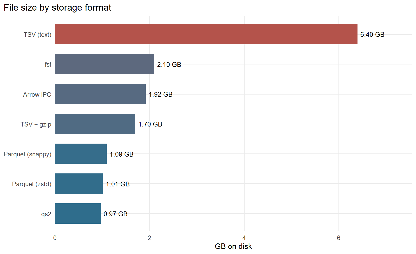
4.1 What Parquet actually buys you
Parquet is a binary, columnar, compressed format. Data is stored column by column rather than row by row, in independently compressed chunks called row groups, each carrying min/max statistics for its columns.
That layout produces three distinct wins, worth separating because only the first is about file size:
- Compression. Values within a column are homogeneous, so they compress far better than a row of mixed types. Snappy decompresses fastest; zstd is noticeably smaller for a little more CPU and is the better default today.
- Projection pushdown. Reading 2 of 15 columns reads roughly 2/15ths of the bytes. A row-oriented format must read every row in full and discard.
- Predicate pushdown. Row-group statistics let a reader skip entire chunks that cannot contain matching rows, without decompressing them.
The last two are properties of the reader, not the file, which is why they show up in the Polars and DuckDB numbers and not the base R ones. Section 5.3 measures them.
The costs are real but narrow: Parquet is not human-readable, the overhead is not worth it for small data, and writes are slower than appending to a CSV.
4.2 .duckdb files versus Parquet
A .duckdb file is DuckDB’s own storage format. Against Parquet it trades portability for query speed: it carries indexes and zone maps, supports transactional updates, and DuckDB queries it faster than it queries Parquet. But only DuckDB reads it, and it is larger.
Parquet for data you share or archive; .duckdb for a working set you query repeatedly. Since DuckDB 1.0 the storage format is stable across versions, so a .duckdb file is no longer a throwaway artifact.
5 Reading data
5.1 Reading text
text_methods <- list(
  bench_method("data.table::fread", "data.table",
               function() data.table::fread(TSV, nThread = params$threads),
               "parallel C parser"),
  bench_method("vroom (ALTREP, lazy)", "tidyverse",
               function() vroom::vroom(TSV, delim = "\t", show_col_types = FALSE,
                                       num_threads = params$threads),
               "builds an index only"),
  bench_method("vroom (materialized)", "tidyverse",
               function() vroom::vroom(TSV, delim = "\t", show_col_types = FALSE,
                                       num_threads = params$threads, altrep = FALSE),
               "forced to read every column"),
  bench_method("readr::read_delim", "tidyverse",
               function() readr::read_delim(TSV, delim = "\t", show_col_types = FALSE,
                                            num_threads = params$threads), "readr 2.x"),
  bench_method("polars scan_csv", "polars",
               function() pl$scan_csv(TSV, separator = "\t")$collect(engine = "streaming"),
               "Rust, multithreaded"),
  bench_method("DuckDB read_csv", "DuckDB",
               function() {
                 cc <- dbConnect(duckdb(), config = list(threads = as.character(params$threads)))
                 on.exit(dbDisconnect(cc, shutdown = TRUE), add = TRUE)
                 dbGetQuery(cc, sprintf("SELECT * FROM read_csv('%s', delim='\t', header=true)", TSV))
               }, "parallel CSV sniffer")
)
if (isTRUE(params$run_read_table)) {
  text_methods <- c(list(bench_method("base R read.table", "base R",
    function() utils::read.table(TSV, header = TRUE, sep = "\t", quote = "\""),
    "the baseline")), text_methods)
}
read_res <- run_suite(text_methods, sample_mem = TRUE)
read_res |>
  transform(GB_per_s = (file.size(TSV)/GB) / elapsed) |>
  subset(select = c(method, note, elapsed, peak_gb, parallelism, GB_per_s)) |>
  kable(digits = 2, caption = sprintf("Reading a %.1f GB tab-separated file", file.size(TSV)/GB),
col.names = c("Method", "Note", "Elapsed (s)", "Peak RSS (GB)", "CPU/wall", "GB/s"))| Method | Note | Elapsed (s) | Peak RSS (GB) | CPU/wall | GB/s |
|---|---|---|---|---|---|
| base R read.table | the baseline | 296.69 | 19.65 | 1.00 | 0.02 |
| data.table::fread | parallel C parser | 4.08 | 15.06 | 3.72 | 1.60 |
| vroom (ALTREP, lazy) | builds an index only | 3.84 | 16.80 | 7.21 | 1.70 |
| vroom (materialized) | forced to read every column | 15.67 | 21.85 | 4.71 | 0.42 |
| readr::read_delim | readr 2.x | 15.18 | 21.84 | 4.88 | 0.43 |
| polars scan_csv | Rust, multithreaded | 4.91 | 19.19 | 3.83 | 1.33 |
| DuckDB read_csv | parallel CSV sniffer | 6.11 | 17.54 | 4.92 | 1.07 |
WarningThe two
vroom rows are a benchmarking trap
vroom is deliberately lazy: by default it builds an index of where each field starts and returns immediately, materializing a column only when you touch it. The “ALTREP, lazy” row therefore measures index construction, not reading, and looks impossibly fast.
That is not a criticism of vroom, since deferring work you may never need is a good strategy, and if you use three of fifteen columns you never pay for the other twelve. It is a criticism of benchmarking it naively. The “materialized” row passes altrep = FALSE to force a like-for-like comparison, and that is the number to read against fread.
NoteWhy
read.table() is so much slower
It is not merely that the parser is written in R. read.table() reads the file twice by default (once to infer types), builds every column as a growing R vector, and converts strings one at a time through R’s global string cache. fread and the Rust/C++ parsers memory-map the file, split it into chunks, and parse those chunks in parallel straight into typed buffers.
5.2 Reading binary formats
bin_methods <- list(
  bench_method("arrow::read_parquet", "arrow",
               function() as.data.frame(arrow::read_parquet(p("d_snappy.parquet"))), "snappy"),
  bench_method("arrow::read_parquet (zstd)", "arrow",
               function() as.data.frame(arrow::read_parquet(p("d_zstd.parquet"))), "zstd"),
  bench_method("polars read_parquet", "polars",
               function() as.data.frame(pl$read_parquet(p("d_snappy.parquet"))), "Rust reader"),
  bench_method("DuckDB -> data.frame", "DuckDB",
               function() {
                 cc <- dbConnect(duckdb(), config = list(threads = as.character(params$threads)))
                 on.exit(dbDisconnect(cc, shutdown = TRUE), add = TRUE)
                 dbGetQuery(cc, sprintf("SELECT * FROM read_parquet('%s')", p("d_snappy.parquet")))
               }, "via DBI"),
  bench_method("arrow::read_feather", "arrow",
               function() as.data.frame(arrow::read_feather(p("d.arrow"))), "Arrow IPC, lz4"),
  bench_method("fst::read_fst", "other",
               function() fst::read_fst(p("d.fst")), "seekable", needs = "fst"),
  bench_method("qs2::qs_read", "other",
               function() qs2::qs_read(p("d.qs2")), "R serialization", needs = "qs2")
)
bin_methods <- Filter(function(m) all(vapply(m$needs, have_pkg, logical(1))), bin_methods)
run_suite(bin_methods, sample_mem = TRUE) |>
  subset(select = c(method, note, elapsed, peak_gb, parallelism)) |>
  kable(digits = 2, caption = "Reading the same data from binary formats",
col.names = c("Method", "Note", "Elapsed (s)", "Peak RSS (GB)", "CPU/wall"))| Method | Note | Elapsed (s) | Peak RSS (GB) | CPU/wall |
|---|---|---|---|---|
| arrow::read_parquet | snappy | 3.97 | 12.41 | 1.00 |
| arrow::read_parquet (zstd) | zstd | 4.21 | 17.72 | 0.99 |
| polars read_parquet | Rust reader | 11.50 | 18.59 | 1.18 |
| DuckDB -> data.frame | via DBI | 3.78 | 20.14 | 2.48 |
| arrow::read_feather | Arrow IPC, lz4 | 0.81 | 17.89 | 3.80 |
| fst::read_fst | seekable | 3.30 | 13.94 | 1.73 |
| qs2::qs_read | R serialization | 5.21 | 13.93 | 0.99 |
Tip
fst and qs2 for R-native storage
fst is fast, compressed, random-access storage for R data frames. It can seek to a row range without decompressing everything before it. qs2 does the same job for arbitrary R objects, not just rectangular tables.
Their limitation is the flip side of their design: they store R’s own types, so only R reads them. If your data never leaves R and you want the fastest round-trip of a data frame, they are excellent. If anyone else needs to read it, use Parquet.
5.3 Projection and predicate pushdown
Where columnar storage stops being a file-size story. The same data, asked three ways:
# All three use the same engine (Polars) so that the only thing varying is how
# much of the file the reader is allowed to skip.
pq_file <- p("d_snappy.parquet")
push <- list(
  bench_method("All 15 columns, all rows", "polars",
               function() as.data.frame(pl$scan_parquet(pq_file)$collect(engine = "streaming")),
               "no pushdown"),
  bench_method("2 columns, all rows", "polars",
               function() as.data.frame(pl$scan_parquet(pq_file)$
                 select("samplename", "cluster_id")$collect(engine = "streaming")),
               "projection pushdown"),
  bench_method("2 columns, filtered rows", "polars",
               function() as.data.frame(pl$scan_parquet(pq_file)$
                 select("samplename", "cluster_id")$
                 filter(pl$col("cluster_id") == 0L)$collect(engine = "streaming")),
               "projection + predicate")
)
run_suite(push, sample_mem = TRUE) |> subset(select = c(method, note, elapsed, peak_gb)) |>
  kable(digits = 2, caption = "You pay for the columns you read, not the columns you have",
col.names = c("Query", "Optimization", "Elapsed (s)", "Peak RSS (GB)"))| Query | Optimization | Elapsed (s) | Peak RSS (GB) |
|---|---|---|---|
| All 15 columns, all rows | no pushdown | 11.00 | 13.25 |
| 2 columns, all rows | projection pushdown | 4.65 | 10.13 |
| 2 columns, filtered rows | projection + predicate | 3.78 | 9.88 |
These deliberately return different answers, so correctness is not compared here. Holding the engine fixed matters: comparing Arrow’s reader against Polars’ would confound “how much did pushdown save” with “which library is faster”.
You can watch the optimizer do it. Polars will show you the plan before and after optimization:
lazy_q <- pl$scan_parquet(PQ)$
  select("samplename", "cluster_id")$
  filter(pl$col("cluster_id") == 0L)

cat("--- as written ---------------------------------------------\n")
--- as written ---------------------------------------------cat(lazy_q$explain(optimized = FALSE))FILTER [(col("cluster_id")) == (0)]
FROM
SELECT [col("samplename"), col("cluster_id")]
Parquet SCAN [fake_pcawg_all.parquet]
PROJECT */15 COLUMNS
ESTIMATED ROWS: 46115588cat("\n\n--- after optimization --------------------------------------\n")
--- after optimization --------------------------------------cat(lazy_q$explain())Parquet SCAN [fake_pcawg_all.parquet]
PROJECT 2/15 COLUMNS
SELECTION: [(col("cluster_id")) == (0)]
ESTIMATED ROWS: 46115588Read these bottom-up. In the optimized plan the projection has been pushed into the Parquet scan itself (PROJECT 2/15 COLUMNS) and the filter has become part of the scan rather than a separate pass over materialized data.
6 Partitioning
You are not limited to one file. A Hive-partitioned dataset splits rows into a directory tree named by the partitioning column:
dataset/chromosome=1/part-0.parquet
dataset/chromosome=2/part-0.parquet
...
The partition column lives in the path rather than inside the files, and a query filtering on it can skip whole directories without opening them. Arrow, Polars and DuckDB all read this layout natively, and it is the standard for data lakes.
It is also the feature people most often misuse, so this section builds three versions of the same data and measures all of them.
part_root <- file.path(tempdir(), "partitioning"); unlink(part_root, recursive = TRUE)
dir.create(part_root, recursive = TRUE)
d_part <- as.data.frame(arrow::read_parquet(PQ))

dirsize <- function(p) sum(file.info(list.files(p, recursive = TRUE, full.names = TRUE))$size,
                           na.rm = TRUE)
nfiles  <- function(p) length(list.files(p, recursive = TRUE))

build <- function(label, cols) {
  path <- file.path(part_root, label)
  t <- measure(arrow::write_dataset(d_part, path, partitioning = cols, format = "parquet"),
               sample_mem = FALSE)$elapsed
  data.frame(layout = label, write_s = t, files = nfiles(path),
             size_gb = dirsize(path)/GB, path = path, stringsAsFactors = FALSE)
}

layouts <- rbind(
  data.frame(layout = "single file", write_s = NA_real_, files = 1L,
             size_gb = file.size(PQ)/GB, path = PQ, stringsAsFactors = FALSE),
  build("by chromosome", "chromosome"),
  build("by samplename", "samplename")
)
rm(d_part); gc(full = TRUE)
used (Mb) gc trigger (Mb) max used (Mb)
Ncells 2436502 130.2 6551488 349.9 2632423 140.6
Vcells 578630339 4414.6 1807570098 13790.7 1086411334 8288.7layouts |> transform(rows_per_file = round(shape$rows / files)) |>
subset(select = c(layout, files, rows_per_file, size_gb, write_s)) |>
kable(digits = 2, caption = "Three physical layouts of identical data",
col.names = c("Layout", "Files", "Rows per file", "Size (GB)", "Write (s)"))| Layout | Files | Rows per file | Size (GB) | Write (s) |
|---|---|---|---|---|
| single file | 1 | 46115588 | 1.10 | NA |
| by chromosome | 22 | 2096163 | 1.79 | 9.61 |
| by samplename | 2778 | 16600 | 1.33 | 14.74 |
Note what partitioning by samplename has already cost before a single query has run: it produced 2778 files instead of one, took longer to write, and occupies more disk than the single file. Compression works within a file, and a few thousand small files compress worse than one large one. Each also carries its own Parquet footer and schema.
6.1 Three queries, three different winners
The whole question is whether a query filters on the partition column.
con_t <- dbConnect(duckdb())
target_sample <- dbGetQuery(
  con_t, sprintf("SELECT samplename FROM read_parquet('%s') LIMIT 1", PQ))$samplename
dbDisconnect(con_t, shutdown = TRUE)

q_one_sample <- function(src) arrow::open_dataset(src) |>
  filter(samplename == target_sample) |> count() |> collect()
q_one_chrom  <- function(src) arrow::open_dataset(src) |>
  filter(chromosome == 1L) |> count() |> collect()
q_full_scan  <- function(src) arrow::open_dataset(src) |>
  group_by(samplename, cluster_id) |> summarize(n = n(), .groups = "drop") |> collect() |> nrow()

grid <- expand.grid(layout = layouts$layout,
                    query  = c("one sample", "one chromosome", "full scan (sMF)"),
                    stringsAsFactors = FALSE)
grid$elapsed <- mapply(function(lay, qry) {
  src <- layouts$path[layouts$layout == lay]
  f <- switch(qry, "one sample" = q_one_sample, "one chromosome" = q_one_chrom,
              "full scan (sMF)" = q_full_scan)
  tryCatch(measure(f(src), sample_mem = FALSE)$elapsed, error = function(e) NA_real_)
}, grid$layout, grid$query)

tidyr::pivot_wider(grid, names_from = query, values_from = elapsed) |>
kable(digits = 3, caption = "Elapsed seconds. Partitioning helps exactly one of these three.")| layout | one sample | one chromosome | full scan (sMF) |
|---|---|---|---|
| single file | 2.20 | 2.31 | 1.11 |
| by chromosome | 1.36 | 0.15 | 1.72 |
| by samplename | 0.15 | 1.45 | 1.71 |
grid |>
  transform(layout = factor(layout, levels = layouts$layout)) |>
  ggplot(aes(layout, elapsed, fill = layout)) +
  geom_col(width = .65) +
  geom_text(aes(label = sprintf("%.2fs", elapsed)), vjust = -0.4, size = 3.2) +
  facet_wrap(~ query, scales = "free_y") +
  scale_fill_manual(values = c("single file" = "#8A8A8A", "by chromosome" = "#2F6D8C",
                               "by samplename" = "#B4534B")) +
  scale_y_continuous(expand = expansion(mult = c(0, .18))) +
  theme(axis.text.x = element_text(angle = 20, hjust = 1)) +
  labs(title = "Query time by physical layout", x = NULL, y = "Seconds")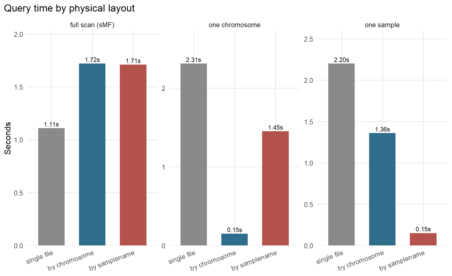
ImportantReading the table
Partitioning by samplename is a trade rather than a mistake, and the trade is usually bad.
For “fetch one sample” it wins enormously: the reader opens one small file instead of scanning the whole dataset. If your actual workload is a per-sample lookup service, this layout is correct and you should use it.
For everything else it loses. The full-scan sMF query, which is the analysis this document is built around, gets slower, because the engine must now open, parse and combine thousands of files, each with its own footer, instead of streaming through one well-organized file with 44 row groups. You also paid more disk and a slower write for the privilege.
The decisive question is not “is my column important?” but “do my queries filter on it?” chromosome is a good partition key because filtering by chromosome is routine, and 22 partitions still leaves each file large enough to be efficient. samplename is a poor one because the common analysis groups across all samples rather than selecting one.
6.2 Where it gets much worse
samplename gives 2,778 partitions, which is bad but survivable, since each file still holds thousands of rows. The failure mode gets much worse as partitions shrink. Partitioning by samplename and chromosome is the kind of thing that looks reasonable in a planning meeting and is a disaster on disk.
Because building it takes three minutes, that chunk is disabled by default and the figures below come from a separate run of all four layouts together. Times are therefore not directly comparable with the live table above, but they are comparable with each other, which is the point:
| Layout | Files | Mean file | Size | Write | Full scan | sMF query |
|---|---|---|---|---|---|---|
| single file | 1 | 1.1 GB | 1.10 GB | n/a | 2.5 s | 1.0 s |
| by chromosome | 22 | 83 MB | 1.79 GB | 3.9 s | 2.5 s | 1.8 s |
| by samplename | 2,778 | 0.5 MB | 1.33 GB | 9.2 s | 1.2 s | 1.6 s |
| samplename × chromosome | 89,303 | 26 KB | 2.18 GB | 182 s | 12.8 s | 11.7 s |
Every column gets worse at once. The dataset takes twice the disk of a single file, takes three minutes to write instead of four seconds, and the analysis it was supposed to accelerate runs eleven times slower. At 26 KB per file you are no longer doing analytics, you are doing filesystem operations: each query pays ~89,000 file opens, Parquet footers and schemas start to rival the data in size, and on cloud object storage you would be billed per request for every one of them.
path_bad <- file.path(part_root, "by_sample_chrom")
d_bad <- as.data.frame(arrow::read_parquet(PQ))
mb <- measure(arrow::write_dataset(d_bad, path_bad,
                                   partitioning = c("samplename", "chromosome"),
                                   format = "parquet"), sample_mem = FALSE)
rm(d_bad); gc(full = TRUE)
data.frame(layout = "by samplename x chromosome", files = nfiles(path_bad),
           mean_file_kb = dirsize(path_bad)/nfiles(path_bad)/1024,
           size_gb = dirsize(path_bad)/GB, write_s = mb$elapsed,
           full_scan_s = measure(q_full_scan(path_bad), sample_mem = FALSE)$elapsed) |>
  kable(digits = 2, caption = "Over-partitioning: same data, ~61,000 files")
WarningThat chunk is off by default
run_pathological: false in the params block, because writing 89,000 small files takes three minutes and is unkind to your filesystem. Set it to true to reproduce the row above; the numbers in the table were measured that way.
A rule of thumb. Aim for partitions of at least a few hundred megabytes, and for no more than a few hundred partitions unless you have a specific reason. If dividing your row count by your partition count leaves you with thousands of rows per file rather than millions, you have gone too far.
And a sanity check before you partition at all: write down the query you are optimizing for. If you cannot name one that filters on the partition column, the answer is a single well-sorted Parquet file. It is faster than every partitioned layout above at the analysis this document actually performs.
These layouts are kept on disk for now: Section 7 benchmarks the full sMF analysis against each of them, so the cost of a partitioning decision shows up in the headline comparison rather than only in a section about partitioning.
7 Workflow 1: subclonal mutation fraction
This is the headline benchmark. Every method below runs in a fresh R process and is timed from nothing: start R, attach packages, get the data, compute the answer. No method inherits a loaded data frame from another.
Code
cold_methods <- list(

  list(label = "base R (aggregate)", family = "base R", note = "read + ave + aggregate",
       pkgs = "arrow", fn = function(pq, threads) {
         d   <- as.data.frame(arrow::read_parquet(pq))
         cl  <- ave(d$cluster_id, d$samplename, FUN = min)
         isc <- d$cluster_id == cl
         a <- aggregate(list(n_snvs   = d$cluster_id),
                        by = list(samplename = d$samplename), FUN = length)
         b <- aggregate(list(n_clonal = isc),
                        by = list(samplename = d$samplename), FUN = sum)
         r <- merge(a, b, by = "samplename")
         r$n_subclonal <- r$n_snvs - r$n_clonal
         r$sMF         <- r$n_subclonal / r$n_snvs
         r }),

  list(label = "dplyr", family = "tidyverse", note = "read + grouped summarize",
       pkgs = c("arrow", "dplyr"), fn = function(pq, threads) {
         as.data.frame(arrow::read_parquet(pq)) |>
           dplyr::summarize(n_snvs   = dplyr::n(),
                            n_clonal = sum(cluster_id == min(cluster_id)),
                            .by = samplename) |>
           dplyr::mutate(n_subclonal = n_snvs - n_clonal, sMF = n_subclonal / n_snvs) }),

  list(label = "data.table", family = "data.table", note = "read + by=",
       pkgs = c("arrow", "data.table"), fn = function(pq, threads) {
         dt <- data.table::as.data.table(arrow::read_parquet(pq))
         r  <- dt[, .(n_snvs = .N, n_clonal = sum(cluster_id == min(cluster_id))),
                  by = samplename]
         r[, `:=`(n_subclonal = n_snvs - n_clonal,
                  sMF = (n_snvs - n_clonal) / n_snvs)][] }),

  list(label = "collapse", family = "collapse", note = "read + C-level grouped stats",
       pkgs = c("arrow", "collapse"), fn = function(pq, threads) {
         d  <- as.data.frame(arrow::read_parquet(pq))
         cl <- collapse::fmin(d$cluster_id, g = d$samplename, TRA = "replace")
         n1 <- collapse::fnobs(d$cluster_id, g = d$samplename)
         n2 <- collapse::fsum(d$cluster_id == cl, g = d$samplename)
         data.frame(samplename = names(n1), n_snvs = as.numeric(n1),
                    n_clonal = as.numeric(n2), n_subclonal = as.numeric(n1 - n2),
                    sMF = as.numeric((n1 - n2) / n1)) }),

  list(label = "arrow (Acero)", family = "arrow", note = "two-stage, never fully in R",
       pkgs = c("arrow", "dplyr"), fn = function(pq, threads) {
         arrow::open_dataset(pq) |>
           dplyr::group_by(samplename, cluster_id) |>
           dplyr::summarize(n = dplyr::n(), .groups = "drop") |>
           dplyr::collect() |>
           dplyr::group_by(samplename) |>
           dplyr::summarize(n_snvs = sum(n), n_clonal = n[which.min(cluster_id)],
                            .groups = "drop") |>
           dplyr::mutate(n_subclonal = n_snvs - n_clonal, sMF = n_subclonal / n_snvs) }),

  list(label = "polars (eager)", family = "polars", note = "read into Polars, then compute",
       pkgs = "polars", fn = function(pq, threads) {
         polars::pl$read_parquet(pq)$group_by("samplename")$agg(
             polars::pl$len()$alias("n_snvs"),
             (polars::pl$col("cluster_id") ==
                polars::pl$col("cluster_id")$min())$sum()$alias("n_clonal")
           )$with_columns((polars::pl$col("n_snvs") -
                           polars::pl$col("n_clonal"))$alias("n_subclonal")
           )$with_columns((polars::pl$col("n_subclonal") /
                           polars::pl$col("n_snvs"))$alias("sMF")) }),

  list(label = "polars (streaming scan)", family = "polars", note = "never enters R",
       pkgs = "polars", fn = function(pq, threads) {
         polars::pl$scan_parquet(pq)$group_by("samplename")$agg(
             polars::pl$len()$alias("n_snvs"),
             (polars::pl$col("cluster_id") ==
                polars::pl$col("cluster_id")$min())$sum()$alias("n_clonal")
           )$with_columns((polars::pl$col("n_snvs") -
                           polars::pl$col("n_clonal"))$alias("n_subclonal")
           )$with_columns((polars::pl$col("n_subclonal") /
                           polars::pl$col("n_snvs"))$alias("sMF")
           )$collect(engine = "streaming") }),

  list(label = "tidypolars", family = "polars", note = "dplyr syntax, Polars engine",
       pkgs = c("polars", "tidypolars", "dplyr"), fn = function(pq, threads) {
         polars::pl$scan_parquet(pq) |>
           dplyr::group_by(samplename) |>
           dplyr::summarize(n_snvs = dplyr::n(),
                            n_clonal = sum(cluster_id == min(cluster_id))) |>
           dplyr::mutate(n_subclonal = n_snvs - n_clonal, sMF = n_subclonal / n_snvs) |>
           dplyr::collect() }),

  list(label = "DuckDB (Parquet, single file)", family = "DuckDB",
       note = "1 file, never enters R",
       pkgs = c("DBI", "duckdb"), fn = function(pq, threads) {
         cc <- DBI::dbConnect(duckdb::duckdb(),
                              config = list(threads = as.character(threads)))
         on.exit(DBI::dbDisconnect(cc, shutdown = TRUE), add = TRUE)
         DBI::dbGetQuery(cc, sprintf("
           SELECT samplename,
                  COUNT(*)                              AS n_snvs,
                  COUNT(*) FILTER (cluster_id = mn)      AS n_clonal,
                  COUNT(*) - COUNT(*) FILTER (cluster_id = mn) AS n_subclonal,
                  (COUNT(*) - COUNT(*) FILTER (cluster_id = mn))::DOUBLE
                    / COUNT(*)                          AS sMF
           FROM (SELECT samplename, cluster_id,
                        MIN(cluster_id) OVER (PARTITION BY samplename) mn
                 FROM read_parquet('%s'))
           GROUP BY ALL", pq)) }),

  list(label = "duckplyr", family = "DuckDB", note = "dplyr syntax, DuckDB engine",
       pkgs = c("duckplyr", "dplyr"), fn = function(pq, threads) {
         duckplyr::read_parquet_duckdb(pq) |>
           dplyr::summarize(n = dplyr::n(), .by = c(samplename, cluster_id)) |>
           dplyr::mutate(mn = min(cluster_id), .by = samplename) |>
           dplyr::summarize(n_snvs = sum(n),
                            n_clonal = sum(ifelse(cluster_id == mn, n, 0)),
                            .by = samplename) |>
           dplyr::mutate(n_subclonal = n_snvs - n_clonal, sMF = n_subclonal / n_snvs) |>
           dplyr::collect() })
)

# --- the same engine over the three physical layouts from @sec-partition ------
# Holding the engine fixed (DuckDB) means the only thing varying is how the bytes
# are arranged on disk.
duck_on_hive <- function(pq, threads) {
  cc <- DBI::dbConnect(duckdb::duckdb(), config = list(threads = as.character(threads)))
  on.exit(DBI::dbDisconnect(cc, shutdown = TRUE), add = TRUE)
  src <- sprintf("read_parquet('%s/**/*.parquet', hive_partitioning = true)",
                 gsub("\\\\", "/", pq))
  DBI::dbGetQuery(cc, sprintf("
    SELECT samplename,
           COUNT(*)                                    AS n_snvs,
           COUNT(*) FILTER (cluster_id = mn)            AS n_clonal,
           COUNT(*) - COUNT(*) FILTER (cluster_id = mn) AS n_subclonal,
           (COUNT(*) - COUNT(*) FILTER (cluster_id = mn))::DOUBLE
             / COUNT(*)                                AS sMF
    FROM (SELECT samplename, cluster_id,
                 MIN(cluster_id) OVER (PARTITION BY samplename) mn
          FROM %s)
    GROUP BY ALL", src))
}

for (lay in c("by chromosome", "by samplename")) {
  cold_methods <- c(cold_methods, list(list(
    label  = paste0("DuckDB (Parquet, ", lay, ")"),
    family = "DuckDB",
    note   = sprintf("%s files", format(layouts$files[layouts$layout == lay], big.mark = ",")),
    pkgs   = c("DBI", "duckdb"),
    pq     = layouts$path[layouts$layout == lay],
    fn     = duck_on_hive)))
}

# The .duckdb-file method only makes sense when that file matches the current scale
if (file.exists(DB)) {
  cold_methods <- c(cold_methods, list(
    list(label = "DuckDB (.duckdb file)", family = "DuckDB", note = "native storage",
         pkgs = c("DBI", "duckdb"), extra = list(dbfile = DB),
         fn = function(pq, threads, dbfile) {
           cc <- DBI::dbConnect(duckdb::duckdb(), dbfile, read_only = TRUE,
                                config = list(threads = as.character(threads)))
           on.exit(DBI::dbDisconnect(cc, shutdown = TRUE), add = TRUE)
           DBI::dbGetQuery(cc, "
             SELECT samplename,
                    COUNT(*)                              AS n_snvs,
                    COUNT(*) FILTER (cluster_id = mn)      AS n_clonal,
                    COUNT(*) - COUNT(*) FILTER (cluster_id = mn) AS n_subclonal,
                    (COUNT(*) - COUNT(*) FILTER (cluster_id = mn))::DOUBLE
                      / COUNT(*)                          AS sMF
             FROM (SELECT samplename, cluster_id,
                          MIN(cluster_id) OVER (PARTITION BY samplename) mn
                   FROM pcawg_all)
             GROUP BY ALL") })))
}
cold_res <- run_cold_suite(cold_methods, pq = PQ, threads = params$threads)cold_res |>
(\(x) x[order(x$elapsed), ])() |>
transform(speedup = max(elapsed, na.rm = TRUE) / elapsed) |>
subset(select = c(method, family, elapsed, speedup, work_s, peak_gb, correct)) |>
kable(digits = 2, row.names = FALSE,
caption = "End-to-end: fresh R process, read the data, compute sMF",
col.names = c("Method", "Family", "Total (s)", "Speedup", "Work (s)",
"Peak RSS (GB)", "Correct"))| Method | Family | Total (s) | Speedup | Work (s) | Peak RSS (GB) | Correct |
|---|---|---|---|---|---|---|
| DuckDB (Parquet, single file) | DuckDB | 0.51 | 70.06 | 0.19 | 0.15 | match |
| DuckDB (.duckdb file) | DuckDB | 0.54 | 66.17 | 0.20 | 0.29 | match |
| duckplyr | DuckDB | 0.87 | 41.07 | 0.33 | 0.17 | match |
| polars (streaming scan) | polars | 0.98 | 36.46 | 0.74 | 2.84 | match |
| DuckDB (Parquet, by samplename) | DuckDB | 1.22 | 29.29 | 0.89 | 0.28 | match |
| tidypolars | polars | 1.25 | 28.58 | 0.79 | 2.93 | match |
| arrow (Acero) | arrow | 1.58 | 22.61 | 1.08 | 0.44 | match |
| polars (eager) | polars | 1.62 | 22.06 | 1.28 | 10.29 | match |
| DuckDB (Parquet, by chromosome) | DuckDB | 3.44 | 10.39 | 3.11 | 1.10 | match |
| collapse | collapse | 7.02 | 5.09 | 6.46 | 7.91 | match |
| dplyr | tidyverse | 7.05 | 5.07 | 6.50 | 7.91 | match |
| data.table | data.table | 9.30 | 3.84 | 8.86 | 13.94 | match |
| base R (aggregate) | base R | 35.73 | 1.00 | 35.30 | 8.29 | reference |
cold_res |> subset(!is.na(elapsed)) |>
  (\(x) transform(x, method = factor(method, levels = x$method[order(-x$elapsed)])))() |>
  ggplot(aes(elapsed, method, fill = family)) +
  geom_col(width = .7) +
  geom_text(aes(label = sprintf("%.1fs", elapsed)), hjust = -0.15, size = 3.3) +
  scale_fill_manual(values = fam_pal) +
  scale_x_continuous(expand = expansion(mult = c(0, .16))) +
  labs(title = "End-to-end time to compute sMF",
       subtitle = sprintf("%s rows, %s samples, %d threads, cold start",
                          format(shape$rows, big.mark = ","),
                          format(shape$samples, big.mark = ","), params$threads),
       x = "Elapsed seconds", y = NULL)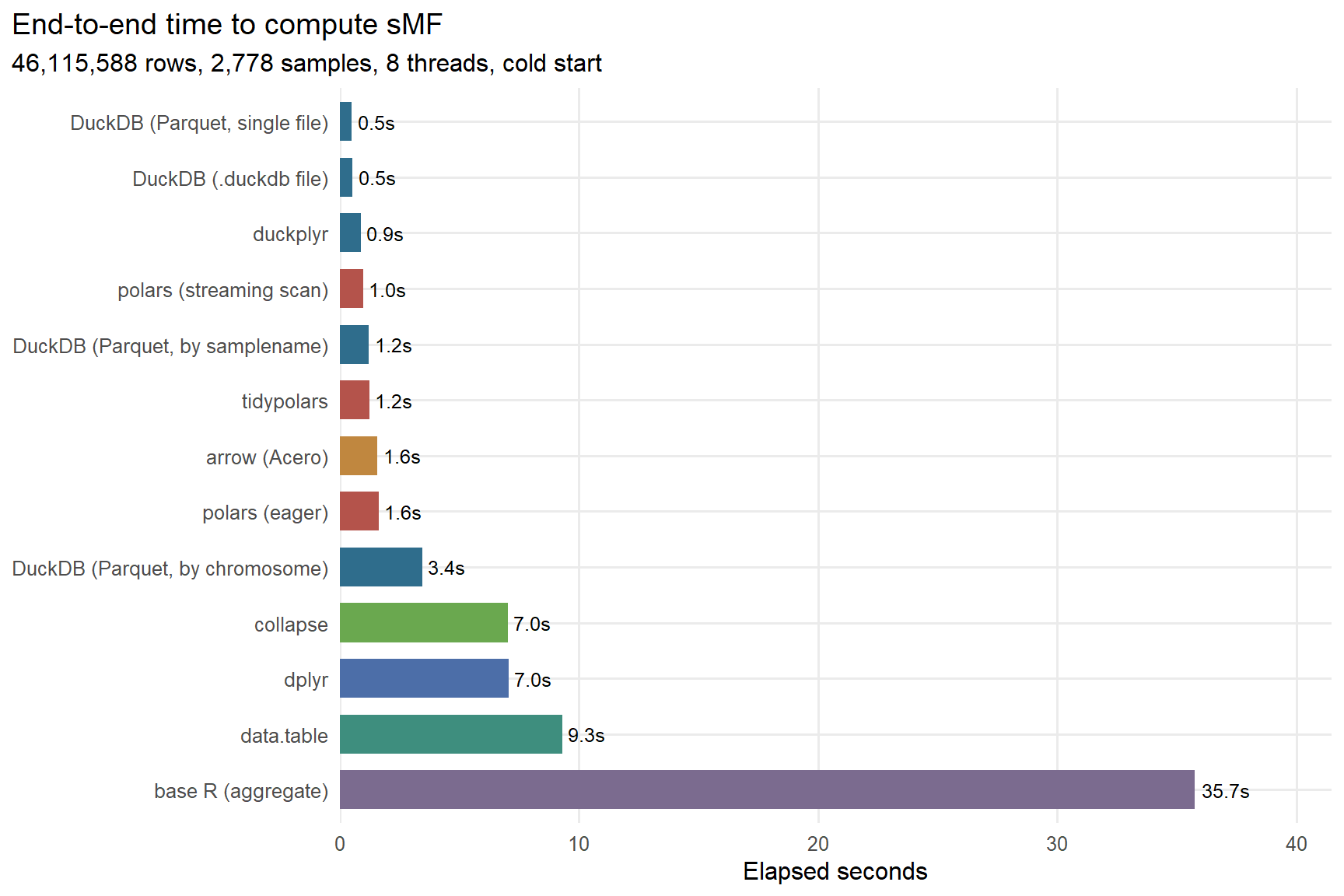
cold_res |> subset(!is.na(peak_gb)) |>
  (\(x) transform(x, method = factor(method, levels = x$method[order(-x$peak_gb)])))() |>
  ggplot(aes(peak_gb, method, fill = family)) +
  geom_col(width = .7) +
  geom_text(aes(label = sprintf("%.2f GB", peak_gb)), hjust = -0.12, size = 3.3) +
  scale_fill_manual(values = fam_pal) +
  scale_x_continuous(expand = expansion(mult = c(0, .2))) +
  labs(title = "Peak process memory, cold start", x = "Peak RSS (GB)", y = NULL)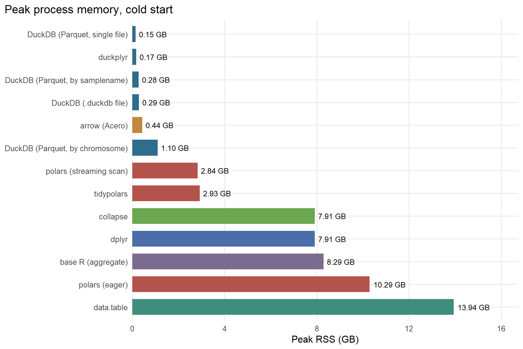
cold_res |> subset(!is.na(elapsed) & !is.na(peak_gb)) |>
  ggplot(aes(elapsed, peak_gb, color = family, label = method)) +
  geom_point(size = 3.2, alpha = .85) +
  ggrepel::geom_text_repel(size = 3, max.overlaps = 20, seed = 1) +
  scale_color_manual(values = fam_pal) +
  scale_x_log10() + scale_y_log10() +
  labs(title = "The actual trade-off", x = "Elapsed seconds (log)",
       y = "Peak RSS, GB (log)")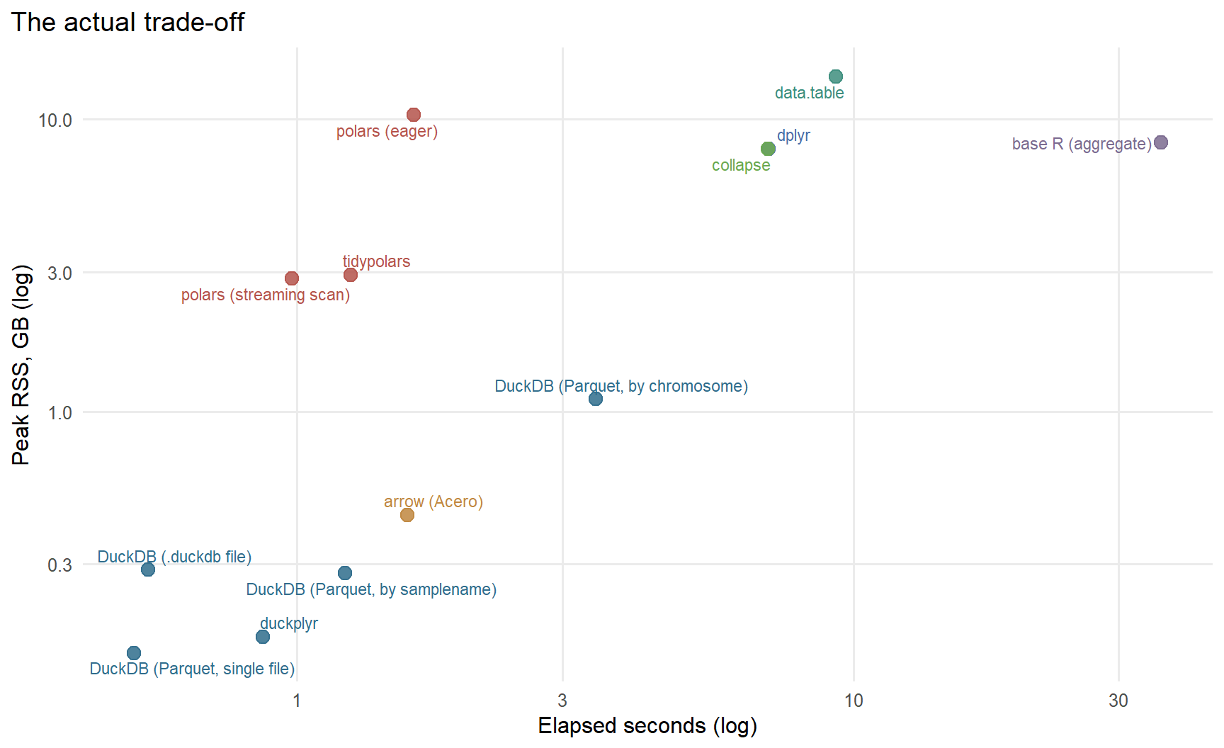
7.1 What the cold-start numbers show
Three things, in decreasing order of importance.
The engines that never load the data win on both axes at once. DuckDB and Polars read the Parquet file, do the aggregation inside their own engine, and hand R back a table of a few thousand rows. Nothing else in the pipeline ever sees 46 million rows. They are both the fastest and the lightest, and it is not close.
Most of the time in the in-memory methods is reading, not computing. Compare the total against the Work (s) column: for dplyr, collapse and data.table the grouped aggregation itself is quick, and they are all perfectly good at that, but they must first materialize the entire table as R objects. That cost is paid before any analysis begins, and it dominates.
Base R is slow for a specific, fixable reason. aggregate() builds and splits large intermediate structures per group. collapse performs the identical calculation on the identical in-memory data frame far faster, which shows the gap is the implementation of the grouped operation and not “R being slow”.
Layout costs as much as library choice. The three DuckDB (Parquet, …) rows are the same engine running the same SQL over the same rows, differing only in how those rows are arranged on disk: one file, 22 files, or 2,778 files. The single file wins. Partitioning is a real cost here, not a rounding error, and it is being paid by a query that never filters on the partition column, which is the situation Section 6 warns about, now visible in the headline table rather than tucked away in a section about storage.
There is also a further lesson hiding inside the Polars rows, and it is the cleanest demonstration in this document that how you ask matters as much as what you ask. polars (eager) and polars (streaming scan) are the same library computing the same answer. The eager version calls pl$read_parquet(), which materializes all 46.1 million rows before doing anything; the streaming version calls pl$scan_parquet() and lets the optimizer push the aggregation into the file scan. The difference between them is several-fold in both time and memory, and the change is a single word, from read_ to scan_. If you take one habit from this section, make it that one.
7.2 When the data is already in memory
Cold start is the right default framing, but it is not every situation. If you have already loaded a data frame and want to run twenty different summaries on it, only the compute cost matters. That question has a different answer:
d <- as.data.frame(arrow::read_parquet(PQ))
dt <- as.data.table(d)

warm <- run_suite(list(
  bench_method("base R aggregate", "base R", function() {
    cl <- ave(d$cluster_id, d$samplename, FUN = min); isc <- d$cluster_id == cl
    a <- aggregate(list(n_snvs = d$cluster_id), by = list(samplename = d$samplename), FUN = length)
    b <- aggregate(list(n_clonal = isc),        by = list(samplename = d$samplename), FUN = sum)
    r <- merge(a, b, by = "samplename")
    r$n_subclonal <- r$n_snvs - r$n_clonal; r$sMF <- r$n_subclonal / r$n_snvs; r }, "in memory"),
  bench_method("dplyr", "tidyverse", function() {
    d |> summarize(n_snvs = n(), n_clonal = sum(cluster_id == min(cluster_id)), .by = samplename) |>
      mutate(n_subclonal = n_snvs - n_clonal, sMF = n_subclonal / n_snvs) }, "in memory"),
  bench_method("data.table", "data.table", function() {
    r <- dt[, .(n_snvs = .N, n_clonal = sum(cluster_id == min(cluster_id))), by = samplename]
    r[, `:=`(n_subclonal = n_snvs - n_clonal, sMF = (n_snvs - n_clonal)/n_snvs)][] }, "in memory"),
  bench_method("collapse", "collapse", function() {
    cl <- fmin(d$cluster_id, g = d$samplename, TRA = "replace")
    n1 <- fnobs(d$cluster_id, g = d$samplename); n2 <- fsum(d$cluster_id == cl, g = d$samplename)
    data.frame(samplename = names(n1), n_snvs = as.numeric(n1), n_clonal = as.numeric(n2),
               n_subclonal = as.numeric(n1-n2), sMF = as.numeric((n1-n2)/n1)) }, "in memory"),
  bench_method("DuckDB (registered df)", "DuckDB", function() {
    cc <- dbConnect(duckdb(), config = list(threads = as.character(params$threads)))
    on.exit(dbDisconnect(cc, shutdown = TRUE), add = TRUE)
    duckdb_register(cc, "rdf", d)
    dbGetQuery(cc, "SELECT samplename, COUNT(*) AS n_snvs,
        COUNT(*) FILTER (cluster_id = mn) AS n_clonal,
        COUNT(*) - COUNT(*) FILTER (cluster_id = mn) AS n_subclonal,
        (COUNT(*) - COUNT(*) FILTER (cluster_id = mn))::DOUBLE / COUNT(*) AS sMF
      FROM (SELECT samplename, cluster_id,
                   MIN(cluster_id) OVER (PARTITION BY samplename) mn FROM rdf)
      GROUP BY ALL") }, "zero-copy view of the R data frame")
), sample_mem = TRUE)

warm |> (\(x) x[order(x$elapsed), ])() |>
  subset(select = c(method, note, elapsed, parallelism, correct)) |>
  kable(digits = 2, row.names = FALSE,
        caption = "Compute only, on a data frame already in memory",
col.names = c("Method", "Note", "Elapsed (s)", "CPU/wall", "Correct"))| Method | Note | Elapsed (s) | CPU/wall | Correct |
|---|---|---|---|---|
| collapse | in memory | 0.35 | 1.06 | match |
| DuckDB (registered df) | zero-copy view of the R data frame | 0.44 | 9.59 | match |
| data.table | in memory | 0.55 | 2.65 | match |
| dplyr | in memory | 0.61 | 0.95 | match |
| base R aggregate | in memory | 16.42 | 1.00 | reference |
On an already-loaded data frame the ranking compresses dramatically and collapse and data.table are genuinely competitive with the query engines, whose advantage was mostly that they avoided the load. Note also duckdb_register(), which exposes an R data frame to DuckDB as a virtual table with no copy, so you can use SQL against data you already have without paying to move it.
8 Workflow 2: annotating variants against gene models
Every result so far has pointed the same way. This one does not, which is why it is here.
Assigning each variant to the gene it falls inside is a range join: match on chromosome and on position BETWEEN gene_start AND gene_end. That inequality changes the algorithm entirely. A hash join, the workhorse of every columnar engine, cannot express “is between”, so the engine must either sort-merge, or fall back to comparing many candidate pairs. Genomics has purpose-built data structures for exactly this (interval and segment trees), and they are hard to beat.
WarningTwo correctness traps
Casting a double to an integer is not the same operation in every engine. The position column is stored as DOUBLE with fractional values, so it has to be made whole before a range join. DuckDB’s CAST(x AS BIGINT) rounds; Polars’ $cast(pl$Int64) truncates:
| position | DuckDB CAST |
Polars $cast |
|---|---|---|
| 74655399.9004755 | 74655400 | 74655399 |
A silent one-base shift, which moves variants across gene boundaries and changes the answer. Every method below uses an explicit FLOOR so they agree.
Polars will not coerce join keys. Joining an Int32 column to an Int64 one raises datatypes of join keys don't match, where SQL and dplyr would quietly promote. That is arguably the better behavior, but it means types have to line up before you join.
Code
overlap_methods <- list(

  list(label = "data.table (foverlaps)", family = "data.table",
       note = "interval tree", pkgs = c("arrow", "data.table"),
       fn = function(pq, threads, genes) {
         v <- data.table::as.data.table(
                as.data.frame(arrow::read_parquet(pq, col_select = c("chromosome", "position"))))
         v[, `:=`(start = as.integer(floor(position)), end = as.integer(floor(position)))]
         v[, position := NULL]
         g <- data.table::as.data.table(as.data.frame(arrow::read_parquet(genes)))
         g <- g[, .(gene_id, chromosome, start = gene_start, end = gene_end)]
         data.table::setkey(g, chromosome, start, end)
         ov <- data.table::foverlaps(v, g, type = "within", nomatch = NULL)
         ov[, .(n_variants = .N), by = gene_id] }),

  list(label = "GenomicRanges", family = "other",
       note = "findOverlaps", pkgs = c("arrow", "GenomicRanges"),
       fn = function(pq, threads, genes) {
         v <- as.data.frame(arrow::read_parquet(pq, col_select = c("chromosome", "position")))
         g <- as.data.frame(arrow::read_parquet(genes))
         hits <- GenomicRanges::findOverlaps(
           GenomicRanges::GRanges(as.character(v$chromosome),
                                  IRanges::IRanges(floor(v$position), width = 1L)),
           GenomicRanges::GRanges(as.character(g$chromosome),
                                  IRanges::IRanges(g$gene_start, g$gene_end)),
           type = "within")
         tab <- table(g$gene_id[S4Vectors::subjectHits(hits)])
         data.frame(gene_id = names(tab), n_variants = as.numeric(tab)) }),

  list(label = "DuckDB (range join)", family = "DuckDB",
       note = "SQL BETWEEN", pkgs = c("DBI", "duckdb"),
       fn = function(pq, threads, genes) {
         cc <- DBI::dbConnect(duckdb::duckdb(),
                              config = list(threads = as.character(threads)))
         on.exit(DBI::dbDisconnect(cc, shutdown = TRUE), add = TRUE)
         DBI::dbGetQuery(cc, sprintf("
           SELECT g.gene_id, COUNT(*) AS n_variants
           FROM (SELECT chromosome, CAST(FLOOR(position) AS BIGINT) AS pos
                 FROM read_parquet('%s')) v
           JOIN read_parquet('%s') g
             ON v.chromosome = g.chromosome
            AND v.pos BETWEEN g.gene_start AND g.gene_end
           GROUP BY ALL", pq, genes)) }),

  list(label = "Polars (join + filter)", family = "polars",
       note = "equi-join then filter", pkgs = "polars",
       fn = function(pq, threads, genes) {
         pv <- polars::pl$scan_parquet(pq)$
                 select("chromosome", "position")$
                 with_columns(polars::pl$col("position")$floor()$
                                cast(polars::pl$Int64)$alias("pos"))$
                 drop("position")
         pg <- polars::pl$scan_parquet(genes)
         as.data.frame(
           pv$join(pg, on = "chromosome", how = "inner")$
             filter((polars::pl$col("pos") >= polars::pl$col("gene_start")) &
                    (polars::pl$col("pos") <= polars::pl$col("gene_end")))$
             group_by("gene_id")$agg(polars::pl$len()$alias("n_variants"))$
             collect(engine = "streaming")) }),

  # --- binned composite key: an equi-join that a range join can hide inside ---
  list(label = "dplyr (binned key)", family = "tidyverse",
       note = "bin, equi-join, filter", pkgs = c("arrow", "dplyr"),
       fn = function(pq, threads, genes) {
         BINSZ <- 10000L
         g  <- as.data.frame(arrow::read_parquet(genes))
         nb <- (g$gene_end %/% BINSZ) - (g$gene_start %/% BINSZ) + 1L
         gb <- data.frame(
           gene_id    = rep(g$gene_id, nb),
           chromosome = rep(g$chromosome, nb),
           gene_start = rep(g$gene_start, nb),
           gene_end   = rep(g$gene_end, nb),
           bin = unlist(mapply(function(a, b) a:b, g$gene_start %/% BINSZ,
                               g$gene_end %/% BINSZ, SIMPLIFY = FALSE), use.names = FALSE))
         v <- as.data.frame(arrow::read_parquet(pq, col_select = c("chromosome", "position")))
         v$pos <- as.integer(floor(v$position)); v$position <- NULL
         v$bin <- v$pos %/% BINSZ
         dplyr::inner_join(v, gb, by = c("chromosome", "bin"),
                           relationship = "many-to-many") |>
           dplyr::filter(pos >= gene_start, pos <= gene_end) |>
           dplyr::summarize(n_variants = dplyr::n(), .by = gene_id) }),

  list(label = "data.table (binned key)", family = "data.table",
       note = "bin, equi-join, filter", pkgs = c("arrow", "data.table"),
       fn = function(pq, threads, genes) {
         BINSZ <- 10000L
         g  <- as.data.frame(arrow::read_parquet(genes))
         nb <- (g$gene_end %/% BINSZ) - (g$gene_start %/% BINSZ) + 1L
         gt <- data.table::data.table(
           gene_id    = rep(g$gene_id, nb),
           chromosome = rep(g$chromosome, nb),
           gene_start = rep(g$gene_start, nb),
           gene_end   = rep(g$gene_end, nb),
           bin = unlist(mapply(function(a, b) a:b, g$gene_start %/% BINSZ,
                               g$gene_end %/% BINSZ, SIMPLIFY = FALSE), use.names = FALSE))
         data.table::setkey(gt, chromosome, bin)
         v <- data.table::as.data.table(as.data.frame(
                arrow::read_parquet(pq, col_select = c("chromosome", "position"))))
         v[, pos := as.integer(floor(position))][, position := NULL][, bin := pos %/% BINSZ]
         m <- gt[v, on = .(chromosome, bin), allow.cartesian = TRUE, nomatch = NULL]
         m[pos >= gene_start & pos <= gene_end, .(n_variants = .N), by = gene_id] })
)
overlap_methods <- lapply(overlap_methods, function(m) { m$extra <- list(genes = GENES); m })
overlap_methods <- Filter(function(m) all(vapply(m$pkgs, have_pkg, logical(1))), overlap_methods)
wf2 <- run_cold_suite(overlap_methods, pq = PQ, threads = params$threads,
canon_fn = canon_generic)
wf2 |> (\(x) x[order(x$elapsed), ])() |>
subset(select = c(method, family, note, elapsed, work_s, peak_gb, correct)) |>
kable(digits = 2, row.names = FALSE,
caption = "Assigning 46M variants to 20,000 genes, cold start",
col.names = c("Method", "Family", "Note", "Total (s)", "Work (s)",
"Peak RSS (GB)", "Correct"))| Method | Family | Note | Total (s) | Work (s) | Peak RSS (GB) | Correct |
|---|---|---|---|---|---|---|
| data.table (binned key) | data.table | bin, equi-join, filter | 3.16 | 2.70 | 2.25 | match |
| dplyr (binned key) | tidyverse | bin, equi-join, filter | 4.18 | 3.70 | 2.33 | match |
| data.table (foverlaps) | data.table | interval tree | 8.81 | 8.40 | 2.24 | reference |
| DuckDB (range join) | DuckDB | SQL BETWEEN | 11.08 | 10.78 | 0.23 | match |
| GenomicRanges | other | findOverlaps | 12.29 | 11.08 | 3.32 | match |
| Polars (join + filter) | polars | equi-join then filter | 133.86 | 133.61 | 1.44 | match |
wf2 |> subset(!is.na(elapsed)) |>
  (\(x) transform(x, method = factor(method, levels = x$method[order(-x$elapsed)])))() |>
  ggplot(aes(elapsed, method, fill = family)) +
  geom_col(width = .65) +
  geom_text(aes(label = sprintf("%.1fs", elapsed)), hjust = -0.15, size = 3.3) +
  scale_fill_manual(values = fam_pal) +
  scale_x_continuous(expand = expansion(mult = c(0, .18))) +
  labs(title = "Variant-to-gene assignment", x = "Elapsed seconds", y = NULL)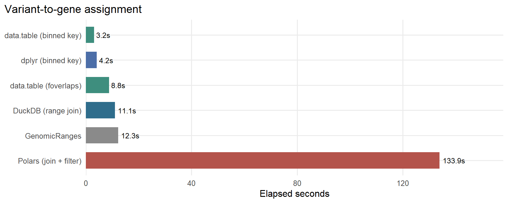
ImportantWhere the column store loses
In Workflow 1 DuckDB beat base R by roughly 70×. Here it does not win at all on time: data.table::foverlaps() matches it, and GenomicRanges is about 11% slower. Only Polars is decisively behind, and by a wide margin.
The reason is structural. foverlaps() and findOverlaps() build an interval index over the (small) gene table and probe it once per variant, roughly n log m. DuckDB must evaluate an inequality predicate, which no hash table can answer. Polars has no interval index at all, so the equi-join on chromosome expands into candidate pairs that are then filtered, doing far more work than either.
The lesson is not “use data.table”. It is that a column store’s advantage comes from scanning and hashing enormous volumes quickly, and a range join is neither a scan nor a hash. When an operation has a purpose-built data structure, the specialized tool is at least competitive, and in genomics ranges come up constantly.
Read the memory column before concluding anything, though: DuckDB does the job in about a tenth of the RAM, because it never materializes the variants in R at all. On time these tools tie; on the resource that actually stops you, they do not.
Polars’ dedicated $join_where() is slower still, not faster: on one chromosome it took 36 s against 5.5 s for the equi-join-then-filter formulation. It is excluded from the table above because at full scale it would dominate the render. If you use it, do not assume the purpose-built verb is the fast path. Measure it.
Note also that GenomicRanges carries an ecosystem the others do not: strand awareness, seqinfo validation, nearest(), distanceToNearest(), coverage. This benchmark measures one narrow operation, not whether the package is worth using.
8.1 The same formulation in base R and dplyr
Polars’ entry above is not a range join. It is an ordinary equi-join on chromosome followed by a filter, the formulation any R user would write first. So the obvious question is what base R and dplyr do with the identical logic.
They cannot run it at all, and the reason is worth working out rather than asserting.
cc <- dbConnect(duckdb(), config = list(threads = as.character(params$threads)))
card <- dbGetQuery(cc, sprintf("
  WITH v AS (SELECT chromosome, COUNT(*) n FROM read_parquet('%s') GROUP BY ALL),
       g AS (SELECT chromosome, COUNT(*) n FROM read_parquet('%s') GROUP BY ALL)
  SELECT SUM(v.n * g.n) AS equijoin_rows FROM v JOIN g USING (chromosome)", PQ, GENES))
dbDisconnect(cc, shutdown = TRUE)
cat(sprintf("rows after joining on chromosome, before filtering: %s (%.1f billion)\n",
            format(card$equijoin_rows, big.mark = ",", scientific = FALSE),
            card$equijoin_rows / 1e9))
rows after joining on chromosome, before filtering: 41,923,257,376 (41.9 billion)cat(sprintf("at a minimal ~36 bytes per row that is about %.1f TB\n",
card$equijoin_rows * 36 / 1024^4))at a minimal ~36 bytes per row that is about 1.4 TBJoining on chromosome alone pairs every variant with every gene on the same chromosome. The filter then throws away all but a tiny fraction, but a data frame has to exist before you can filter it.
Polars survives this because its streaming engine never builds the intermediate: it pulls a batch of variants, joins, filters, aggregates, discards, and repeats, so peak memory is set by the batch rather than by 41.9 billion rows. That is the entire difference, and it is invisible in the source code.
To get a comparable reference we therefore have to shrink the problem until the intermediate fits. Below, all four run on the same 100,000 variants from one chromosome, about 90.9 million intermediate rows instead of 41.9 billion.
naive_pq <- file.path(tempdir(), "wf2_subset.parquet")
cc <- dbConnect(duckdb(), config = list(threads = as.character(params$threads)))
dbExecute(cc, sprintf("
  COPY (SELECT chromosome, CAST(FLOOR(position) AS BIGINT) AS pos
        FROM read_parquet('%s') WHERE chromosome = 22
        ORDER BY pos LIMIT 100000)
  TO '%s' (FORMAT PARQUET)", PQ, gsub("\\\\", "/", naive_pq)))
[1] 1e+05dbDisconnect(cc, shutdown = TRUE)
naive_methods <- list(
list(label = "base R (merge + subset)", family = "base R", note = "materializes the pairs",
pkgs = "arrow", timeout_s = 900, fn = function(pq, threads, genes) {
v <- as.data.frame(arrow::read_parquet(pq))
g <- as.data.frame(arrow::read_parquet(genes))
m <- merge(v, g[, c("gene_id", "chromosome", "gene_start", "gene_end")],
by = "chromosome")
m <- m[m$pos >= m$gene_start & m$pos <= m$gene_end, ]
a <- aggregate(list(n_variants = m$pos), by = list(gene_id = m$gene_id), FUN = length)
a }),
list(label = "dplyr (join + filter)", family = "tidyverse", note = "materializes the pairs",
pkgs = c("arrow", "dplyr"), timeout_s = 900, fn = function(pq, threads, genes) {
v <- as.data.frame(arrow::read_parquet(pq))
g <- as.data.frame(arrow::read_parquet(genes))
dplyr::inner_join(v, g[, c("gene_id", "chromosome", "gene_start", "gene_end")],
by = "chromosome", relationship = "many-to-many") |>
dplyr::filter(pos >= gene_start, pos <= gene_end) |>
dplyr::summarize(n_variants = dplyr::n(), .by = gene_id) }),
list(label = "Polars (join + filter)", family = "polars", note = "streams the pairs",
pkgs = "polars", timeout_s = 900, fn = function(pq, threads, genes) {
as.data.frame(
polars::pl$scan_parquet(pq)$
join(polars::pl$scan_parquet(genes), on = "chromosome", how = "inner")$
filter((polars::pl$col("pos") >= polars::pl$col("gene_start")) &
(polars::pl$col("pos") <= polars::pl$col("gene_end")))$
group_by("gene_id")$agg(polars::pl$len()$alias("n_variants"))$
collect(engine = "streaming")) }),
list(label = "data.table (foverlaps)", family = "data.table", note = "never builds pairs",
pkgs = c("arrow", "data.table"), timeout_s = 900, fn = function(pq, threads, genes) {
v <- data.table::as.data.table(as.data.frame(arrow::read_parquet(pq)))
v[, `:=`(start = pos, end = pos)]
g <- data.table::as.data.table(as.data.frame(arrow::read_parquet(genes)))
g <- g[, .(gene_id, chromosome, start = gene_start, end = gene_end)]
data.table::setkey(g, chromosome, start, end)
data.table::foverlaps(v, g, type = "within",
nomatch = NULL)[, .(n_variants = .N), by = gene_id] })
)
naive_methods <- lapply(naive_methods, function(m) { m$extra <- list(genes = GENES); m })
naive_methods <- Filter(function(m) all(vapply(m$pkgs, have_pkg, logical(1))), naive_methods)
wf2b <- run_cold_suite(naive_methods, pq = naive_pq, threads = params$threads,
canon_fn = canon_generic)
unlink(naive_pq)
wf2b |> (\(x) x[order(x$elapsed), ])() |>
subset(select = c(method, family, note, elapsed, work_s, peak_gb, correct)) |>
kable(digits = 2, row.names = FALSE,
caption = "The identical logic on 100,000 variants (0.2% of the data)",
col.names = c("Method", "Family", "Note", "Total (s)", "Work (s)",
"Peak RSS (GB)", "Correct"))| Method | Family | Note | Total (s) | Work (s) | Peak RSS (GB) | Correct |
|---|---|---|---|---|---|---|
| data.table (foverlaps) | data.table | never builds pairs | 0.47 | 0.05 | 0.16 | match |
| Polars (join + filter) | polars | streams the pairs | 0.59 | 0.35 | 0.17 | match |
| dplyr (join + filter) | tidyverse | materializes the pairs | 5.28 | 4.80 | 3.86 | match |
| base R (merge + subset) | base R | materializes the pairs | 168.85 | 168.50 | 23.16 | reference |
ImportantThe memory column, on 0.2% of the data
All four agree on the answer, and on time the ordering is unsurprising: foverlaps, which never builds the pairs at all, is fastest; base R is slowest by a very wide margin.
The memory column is the alarming one. base R peaked at 23.2 GB, on two hundredths of the dataset. dplyr is far better but still materializes the pairs, at a few gigabytes. Polars, running the same join-then-filter logic, used a fraction of a gigabyte, because the streaming engine never holds the intermediate: it pulls a batch of variants, joins, filters, aggregates, discards, repeats.
Now scale it. The intermediate grows as variants × genes-on-that-chromosome, so going from 100,000 variants to 46.1 million multiplies it by 460×, to 41.9 billion rows and roughly 1.4 TB. base R and dplyr do not become slower at that point; they stop being possible. Polars runs the identical source code over the full dataset in about two minutes (see the table above).
That is the clearest demonstration in this document of what a streaming engine buys you, and it is not that the Rust is fast. It is that an execution model which never materializes the intermediate turns an impossible query into a merely slow one. The same source code is fine or fatal depending entirely on what is underneath it.
8.2 Rescuing the join with a binned key
The natural next thought is: rather than joining on chromosome and filtering, why not build a composite key and join on that? For an exact-match join that works well (Section 10.1). For a range join it cannot work directly, since no equality test expresses “between”, but it points at the fix.
Join on chromosome and a positional bin. Cut the genome into 10 kb windows; a variant belongs to exactly one, and a gene is expanded to the handful it spans. The join is then an ordinary two-column equi-join, and the filter only has to check the few candidates that share a bin instead of every gene on the chromosome.
BINSZ <- 10000L
v$bin  <- v$pos %/% BINSZ                    # one row per variant
gb     <- expand_genes_to_bins(g, BINSZ)     # ~174,000 rows from 20,000 genes
inner_join(v, gb, by = c("chromosome", "bin")) |>
  filter(pos >= gene_start, pos <= gene_end)
The intermediate collapses from 41.9 billion rows to roughly the number of variants. That is a change of about 910×, and it is the reason this idea is worth knowing: it is the same trick UCSC’s genome browser has used for decades.
Both binned implementations are in the main table at the top of this section, so they are directly comparable with everything else.
ImportantThe result
Look at where the two binned rows land: top of the table. data.table with a binned key is the fastest method in the section, and plain dplyr with a binned key comes second, ahead of foverlaps(), ahead of DuckDB’s range join, ahead of GenomicRanges, and about thirty times faster than Polars running the unbinned version of the same logic.
That is worth sitting with, because it cuts against the rest of this document. No new library was installed. The engine did not change. What changed is that the query was reformulated so the work matches what a hash join is good at, using one line of domain knowledge about how genomic coordinates behave.
Algorithmic reformulation beats tool selection. Most of this tutorial is about choosing an engine, because most of the time that is the lever you have. But when you know something about the structure of your problem that the engine cannot infer, using it is worth more than any amount of Rust.
The caveats: binning costs you a parameter (10 kb is arbitrary; too small and the gene table explodes, too large and you are back to filtering many candidates), it assumes intervals that are short relative to the bin, and it is code you now have to maintain and test. foverlaps() and findOverlaps() need none of that and are within a factor of a few. For a one-off analysis, use the interval tools; for something in a hot loop, the bin is worth the parameter.
9 Workflow 3: mutation density in genomic bins
Workflow 1 returned 2,778 rows. That flattered the query engines: their whole advantage was aggregating 46.1 million rows down to something tiny and handing R only the tiny thing. Real analyses are not always so kind.
Counting mutations per sample per 1 Mb window produces millions of output rows, so this workflow tests a part of the pipeline the first one never touched: getting a large result out of the engine and into R.
Code
BIN <- 1e6
density_methods <- list(

  list(label = "DuckDB", family = "DuckDB", note = "SQL GROUP BY",
       pkgs = c("DBI", "duckdb"), fn = function(pq, threads) {
         cc <- DBI::dbConnect(duckdb::duckdb(),
                              config = list(threads = as.character(threads)))
         on.exit(DBI::dbDisconnect(cc, shutdown = TRUE), add = TRUE)
         DBI::dbGetQuery(cc, sprintf("
           SELECT samplename, chromosome,
                  CAST(FLOOR(position / 1000000) AS INTEGER) AS bin,
                  COUNT(*) AS n
           FROM read_parquet('%s') GROUP BY ALL", pq)) }),

  list(label = "Polars (streaming)", family = "polars", note = "scan + group_by",
       pkgs = "polars", fn = function(pq, threads) {
         as.data.frame(polars::pl$scan_parquet(pq)$
           with_columns((polars::pl$col("position") / 1e6)$floor()$
                          cast(polars::pl$Int32)$alias("bin"))$
           group_by("samplename", "chromosome", "bin")$
           agg(polars::pl$len()$alias("n"))$
           collect(engine = "streaming")) }),

  list(label = "data.table", family = "data.table", note = "in-memory by=",
       pkgs = c("arrow", "data.table"), fn = function(pq, threads) {
         dt <- data.table::as.data.table(as.data.frame(arrow::read_parquet(
                 pq, col_select = c("samplename", "chromosome", "position"))))
         dt[, bin := as.integer(floor(position / 1000000))]
         dt[, .(n = .N), by = .(samplename, chromosome, bin)] }),

  list(label = "collapse", family = "collapse", note = "in-memory GRP",
       pkgs = c("arrow", "collapse"), fn = function(pq, threads) {
         d <- as.data.frame(arrow::read_parquet(
                pq, col_select = c("samplename", "chromosome", "position")))
         d$bin <- as.integer(floor(d$position / 1000000))
         g <- collapse::GRP(d[, c("samplename", "chromosome", "bin")])
         cbind(g$groups, n = as.numeric(collapse::GRPN(g, expand = FALSE))) })
)
wf3 <- run_cold_suite(density_methods, pq = PQ, threads = params$threads,
canon_fn = canon_generic)
wf3 |> (\(x) x[order(x$elapsed), ])() |>
subset(select = c(method, family, note, elapsed, work_s, peak_gb, correct)) |>
kable(digits = 2, row.names = FALSE,
caption = "Mutations per sample per 1 Mb bin -- a result with millions of rows",
col.names = c("Method", "Family", "Note", "Total (s)", "Work (s)",
"Peak RSS (GB)", "Correct"))| Method | Family | Note | Total (s) | Work (s) | Peak RSS (GB) | Correct |
|---|---|---|---|---|---|---|
| DuckDB | DuckDB | SQL GROUP BY | 2.33 | 0.94 | 1.27 | reference |
| Polars (streaming) | polars | scan + group_by | 3.30 | 2.09 | 2.61 | match |
| collapse | collapse | in-memory GRP | 5.96 | 4.38 | 3.47 | match |
| data.table | data.table | in-memory by= | 6.70 | 5.21 | 4.81 | match |
n_bins <- attr(wf3, "reference")
cat(sprintf("result rows: %s (Workflow 1 returned %s)\n",
            format(nrow(n_bins), big.mark = ","), format(shape$samples, big.mark = ",")))
result rows: 8,870,305 (Workflow 1 returned 2,778)
NoteThe engines still win, but by less
Compare the speedup spread here with Workflow 1. The query engines remain fastest, but the margin narrows, because a growing share of their time is no longer the aggregation, and is instead serializing a multi-million-row result across the boundary into R’s memory.
The practical rule: aggregate to a small result and the engine’s advantage is enormous; aggregate to a large one and you start paying for the handover. If a large intermediate is only going to feed another query, do not bring it into R at all. Keep it in the engine, or write it straight to Parquet with sink_parquet() or COPY ... TO.
10 Workflow 4: flagging known variants
A routine annotation step: mark which of the 46.1 million observed variants appear in a catalogue of known sites. Our synthetic catalogue has 36.3 million rows, so this is a large-to-large equi-join, the operation most likely to exhaust memory in R.
Code
lookup_methods <- list(

  list(label = "DuckDB", family = "DuckDB", note = "hash join, out-of-core capable",
       pkgs = c("DBI", "duckdb"), fn = function(pq, threads, known) {
         cc <- DBI::dbConnect(duckdb::duckdb(),
                              config = list(threads = as.character(threads)))
         on.exit(DBI::dbDisconnect(cc, shutdown = TRUE), add = TRUE)
         DBI::dbGetQuery(cc, sprintf("
           SELECT v.samplename,
                  COUNT(*)                      AS n_variants,
                  COUNT(k.rsid)                 AS n_known,
                  COUNT(*) - COUNT(k.rsid)      AS n_novel
           FROM (SELECT samplename, chromosome, CAST(FLOOR(position) AS BIGINT) AS pos
                 FROM read_parquet('%s')) v
           LEFT JOIN read_parquet('%s') k
             ON k.chromosome = v.chromosome AND k.pos = v.pos
           GROUP BY ALL", pq, known)) }),

  list(label = "Polars (streaming)", family = "polars", note = "scan both sides",
       pkgs = "polars", fn = function(pq, threads, known) {
         pv <- polars::pl$scan_parquet(pq)$
                 select("samplename", "chromosome", "position")$
                 with_columns(polars::pl$col("position")$floor()$
                                cast(polars::pl$Int64)$alias("pos"))$drop("position")
         pk <- polars::pl$scan_parquet(known)$select("chromosome", "pos", "rsid")
         as.data.frame(
           pv$join(pk, on = c("chromosome", "pos"), how = "left")$
             group_by("samplename")$
             agg(polars::pl$len()$alias("n_variants"),
                 polars::pl$col("rsid")$count()$alias("n_known"))$
             with_columns((polars::pl$col("n_variants") -
                           polars::pl$col("n_known"))$alias("n_novel"))$
             collect(engine = "streaming")) }),

  list(label = "data.table (merge)", family = "data.table", note = "both sides in RAM",
       pkgs = c("arrow", "data.table"), fn = function(pq, threads, known) {
         v <- data.table::as.data.table(as.data.frame(arrow::read_parquet(
                pq, col_select = c("samplename", "chromosome", "position"))))
         v[, pos := as.integer(floor(position))][, position := NULL]
         k <- data.table::as.data.table(as.data.frame(
                arrow::read_parquet(known, col_select = c("chromosome", "pos", "rsid"))))
         data.table::setkey(k, chromosome, pos)
         m <- k[v, on = .(chromosome, pos)]
         m[, .(n_variants = .N, n_known = sum(!is.na(rsid)),
               n_novel = sum(is.na(rsid))), by = samplename] }),

  # --- the two approaches a user is most likely to reach for first ------------
  list(label = "dplyr (left_join)", family = "tidyverse", note = "both sides in RAM",
       pkgs = c("arrow", "dplyr"), timeout_s = 1800,
       fn = function(pq, threads, known) {
         v <- as.data.frame(arrow::read_parquet(
                pq, col_select = c("samplename", "chromosome", "position")))
         v$pos <- as.integer(floor(v$position)); v$position <- NULL
         k <- as.data.frame(arrow::read_parquet(known,
                col_select = c("chromosome", "pos", "rsid")))
         dplyr::left_join(v, k, by = c("chromosome", "pos")) |>
           dplyr::summarize(n_variants = dplyr::n(),
                            n_known = sum(!is.na(rsid)),
                            n_novel = sum(is.na(rsid)), .by = samplename) }),

  list(label = "base R (merge)", family = "base R", note = "sort-based merge",
       pkgs = "arrow", timeout_s = 1800,
       fn = function(pq, threads, known) {
         v <- as.data.frame(arrow::read_parquet(
                pq, col_select = c("samplename", "chromosome", "position")))
         v$pos <- as.integer(floor(v$position)); v$position <- NULL
         k <- as.data.frame(arrow::read_parquet(known,
                col_select = c("chromosome", "pos", "rsid")))
         m <- merge(v, k, by = c("chromosome", "pos"), all.x = TRUE)
         n_tot <- aggregate(list(n_variants = m$pos),
                            by = list(samplename = m$samplename), FUN = length)
         n_kn  <- aggregate(list(n_known = !is.na(m$rsid)),
                            by = list(samplename = m$samplename), FUN = sum)
         r <- merge(n_tot, n_kn, by = "samplename")
         r$n_novel <- r$n_variants - r$n_known
         r }),

  # --- composite single-column keys ------------------------------------------
  list(label = "dplyr (packed integer key)", family = "tidyverse",
       note = "chromosome * 1e9 + pos", pkgs = c("arrow", "dplyr"), timeout_s = 1800,
       fn = function(pq, threads, known) {
         v <- as.data.frame(arrow::read_parquet(
                pq, col_select = c("samplename", "chromosome", "position")))
         v$key <- v$chromosome * 1e9 + floor(v$position)
         k <- as.data.frame(arrow::read_parquet(known,
                col_select = c("chromosome", "pos", "rsid")))
         k$key <- k$chromosome * 1e9 + k$pos
         dplyr::left_join(v[, c("samplename", "key")], k[, c("key", "rsid")],
                          by = "key") |>
           dplyr::summarize(n_variants = dplyr::n(),
                            n_known = sum(!is.na(rsid)),
                            n_novel = sum(is.na(rsid)), .by = samplename) }),

  list(label = "dplyr (pasted string key)", family = "tidyverse",
       note = "paste(chr, pos) -- see callout", pkgs = c("arrow", "dplyr"), timeout_s = 1800,
       fn = function(pq, threads, known) {
         v <- as.data.frame(arrow::read_parquet(
                pq, col_select = c("samplename", "chromosome", "position")))
         v$key <- paste(v$chromosome, floor(v$position), sep = "_")
         k <- as.data.frame(arrow::read_parquet(known,
                col_select = c("chromosome", "pos", "rsid")))
         k$key <- paste(k$chromosome, k$pos, sep = "_")
         dplyr::left_join(v[, c("samplename", "key")], k[, c("key", "rsid")],
                          by = "key") |>
           dplyr::summarize(n_variants = dplyr::n(),
                            n_known = sum(!is.na(rsid)),
                            n_novel = sum(is.na(rsid)), .by = samplename) })
)
lookup_methods <- lapply(lookup_methods, function(m) { m$extra <- list(known = KNOWN); m })
lookup_methods <- Filter(function(m) all(vapply(m$pkgs, have_pkg, logical(1))), lookup_methods)
wf4 <- run_cold_suite(lookup_methods, pq = PQ, threads = params$threads,
canon_fn = canon_generic)
wf4 |> (\(x) x[order(x$elapsed), ])() |>
subset(select = c(method, family, note, elapsed, work_s, peak_gb, correct, status)) |>
kable(digits = 2, row.names = FALSE,
caption = "Joining 46M variants to a 36M-row catalogue",
col.names = c("Method", "Family", "Note", "Total (s)", "Work (s)",
"Peak RSS (GB)", "Correct", "Status"))| Method | Family | Note | Total (s) | Work (s) | Peak RSS (GB) | Correct | Status |
|---|---|---|---|---|---|---|---|
| DuckDB | DuckDB | hash join, out-of-core capable | 1.15 | 0.87 | 2.95 | reference | ok |
| Polars (streaming) | polars | scan both sides | 2.55 | 2.32 | 4.19 | match | ok |
| dplyr (left_join) | tidyverse | both sides in RAM | 24.30 | 23.76 | 8.00 | match | ok |
| dplyr (packed integer key) | tidyverse | chromosome * 1e9 + pos | 24.98 | 24.45 | 7.43 | match | ok |
| data.table (merge) | data.table | both sides in RAM | 40.20 | 39.73 | 6.37 | match | ok |
| dplyr (pasted string key) | tidyverse | paste(chr, pos) – see callout | 267.74 | 267.19 | 14.06 | MISMATCH | ok |
| base R (merge) | base R | sort-based merge | 347.23 | 346.77 | 23.06 | match | ok |
ImportantThe case that breaks laptops
Two large tables joined on a compound key is where an in-memory approach stops being merely slower and starts being a different category of problem. Both sides have to be materialized, the join builds a hash table over one of them, and the peak sits well above the sum of the inputs.
DuckDB and Polars do something structurally different: they stream both sides from Parquet, never materialize either in full, and spill to disk if the hash table outgrows the budget. On a machine with less RAM than this one, the in-memory rows are the ones that fail, and they fail at the end, after you have waited.
The bottom two rows are there deliberately. dplyr::left_join() and base R’s merge() are what most people reach for first, and they are nothing like each other. dplyr uses a hash join and is entirely respectable, and it even beats data.table here. merge() sorts both inputs, and sorting 36.3 million rows is ruinous: it is roughly 14× slower than dplyr and 300× slower than DuckDB.
Look at the memory column, though, because that is the part that actually decides whether your script runs. merge() peaked at 23.1 GB, for a join whose inputs total under half a gigabyte on disk. On a 16 GB laptop this row fails outright.
A further detail from measuring it at smaller sizes: merge()’s cost is dominated by the catalogue, not the variant table, so it barely improves when you shrink the side you control. Sampling your data to make it faster would not have helped.
merge() is a perfectly good function on a thousand rows. The failure is not the function. It is reaching for the familiar one without checking how it scales.
10.1 Composite keys: one column instead of two
A common instinct for a two-column join is to fuse the columns into a single key. It is a reasonable idea, and how you build the key matters enormously.
Packing into an integer is safe, but here it buys nothing. Positions are below 2.5 × 10⁸ and chromosomes below 23, so chromosome * 1e9 + pos is unique and fits comfortably inside a double’s 53 bits of integer precision. Hashing one numeric column is cheaper than hashing two, and yet the packed row above is no faster than the plain two-column join.
That is worth a moment, because on a smaller slice of the same data it clearly is faster. Measured on 6.3 million variants rather than 46 million, the packed key ran in 1.7 s against 3.7 s for the two-column join, a solid 2× win. At full scale the win evaporates: building the key costs a full extra pass over both tables and two new 46-million and 36-million element vectors, which is about what the cheaper hashing saves.
A micro-optimization that helps at one size can be a wash at another. If you are going to fuse keys for speed, measure it at the size you actually run at, not at the size that fits in a quick test.
Pasting into a string is worse than useless. It is an order of magnitude slower than either alternative, since building 46 million strings and hashing them costs far more than the join it was meant to help. It is also wrong, which matters more.
WarningThe pasted key silently loses rows
paste(chromosome, pos, sep = "_") calls as.character() on a numeric column, and R renders large round doubles in scientific notation:
paste0(70000000)    # "7e+07"
paste0(130000000)   # "1.3e+08"
paste0(220000000)   # "2.2e+08"
Three positions in this dataset are affected. Their keys become "22_2.2e+08" instead of "22_220000000", they fail to match the catalogue, and the variant is reported as novel when it is known.
No error, no warning, just a slightly wrong answer, from three positions out of forty-six million. A test on a thousand rows would never catch it, and neither would any amount of timing.
Look at the Correct column for that row in the table above: it reads MISMATCH. That is the only wrong answer anywhere in this document, and it is visible solely because every method is compared against a reference result rather than just timed. A benchmark that reported speed alone would have ranked this implementation and said nothing about it being incorrect.
If you must build a string key, force the representation: sprintf("%d_%.0f", chr, pos) or format(pos, scientific = FALSE). Better, pack it into an integer and skip the whole class of problem.
NoteMethods here run under a timeout
measure_cold(timeout_s =) kills a method that exceeds its budget and records the timeout, so an approach that might never finish cannot stall the document. Both slow rows above are capped at 30 minutes, and both came in under it, so these are real measurements rather than lower bounds. Had one timed out, that would have been the result: an approach that does not finish is unusable rather than slow.
11 Workflow 5: RNAseq QC and normalization
Everything so far has been row-oriented: filter, group, join. Expression analysis is different. A count matrix is genuinely matrix-shaped, and the standard QC steps are linear algebra: library-size normalization, filtering low-expression genes, log transformation, and sample-to-sample correlation for outlier detection.
This is where the tutorial’s thesis has a limit.
cc <- dbConnect(duckdb(), config = list(threads = as.character(params$threads)))
wide_cols <- ncol(dbGetQuery(cc, sprintf("SELECT * FROM read_parquet('%s') LIMIT 0", COUNTS_W)))
long_rows <- dbGetQuery(cc, sprintf("SELECT COUNT(*) n FROM read_parquet('%s')", COUNTS_L))$n
dbDisconnect(cc, shutdown = TRUE)
cat(sprintf("wide: %s genes x %s samples   |   long: %s rows\n",
            format(20000, big.mark = ","), format(wide_cols - 1, big.mark = ","),
            format(long_rows, big.mark = ",")))
wide: 20,000 genes x 2,778 samples | long: 55,560,000 rows11.1 The same matrix, two layouts
The counts are stored twice: long (gene_id, samplename, count) and wide (one row per gene, one column per sample). Which layout is right depends entirely on which way you slice.
key_ids <- c("ENSG00000000101","ENSG00000000202","ENSG00000000303",
             "ENSG00000000404","ENSG00000000505")
con_s <- dbConnect(duckdb())
some_samples <- dbGetQuery(con_s, sprintf(
  "SELECT samplename FROM read_parquet('%s') ORDER BY samplename LIMIT 5", META))$samplename
dbDisconnect(con_s, shutdown = TRUE)

layout_methods <- list(
  bench_method("long: 5 genes, all samples", "DuckDB", function() {
    z <- dbConnect(duckdb(), config = list(threads = as.character(params$threads)))
    on.exit(dbDisconnect(z, shutdown = TRUE), add = TRUE)
    dbGetQuery(z, sprintf("SELECT * FROM read_parquet('%s') WHERE gene_id IN ('%s')",
                          COUNTS_L, paste(key_ids, collapse = "','")))
  }, "predicate pushdown, file sorted by gene"),
  bench_method("wide: 5 genes, all samples", "DuckDB", function() {
    z <- dbConnect(duckdb(), config = list(threads = as.character(params$threads)))
    on.exit(dbDisconnect(z, shutdown = TRUE), add = TRUE)
    dbGetQuery(z, sprintf("SELECT * FROM read_parquet('%s') WHERE gene_id IN ('%s')",
                          COUNTS_W, paste(key_ids, collapse = "','")))
  }, "5 rows -- but every one of 2,778 columns"),
  bench_method("wide: 5 samples, all genes", "DuckDB", function() {
    z <- dbConnect(duckdb(), config = list(threads = as.character(params$threads)))
    on.exit(dbDisconnect(z, shutdown = TRUE), add = TRUE)
    dbGetQuery(z, sprintf('SELECT gene_id, "%s" FROM read_parquet(\'%s\')',
                          paste(some_samples, collapse = '", "'), COUNTS_W))
  }, "projection pushdown: 6 of 2,779 columns"),
  bench_method("long: 5 samples, all genes", "DuckDB", function() {
    z <- dbConnect(duckdb(), config = list(threads = as.character(params$threads)))
    on.exit(dbDisconnect(z, shutdown = TRUE), add = TRUE)
    dbGetQuery(z, sprintf("SELECT * FROM read_parquet('%s') WHERE samplename IN ('%s')",
                          COUNTS_L, paste(some_samples, collapse = "','")))
  }, "no useful sort order: full scan")
)
run_suite(layout_methods, sample_mem = FALSE, canon_fn = canon_generic) |>
  subset(select = c(method, note, elapsed)) |>
  kable(digits = 3, caption = "Long vs wide: the layout decides which questions are cheap",
col.names = c("Query", "Why", "Elapsed (s)"))| Query | Why | Elapsed (s) |
|---|---|---|
| long: 5 genes, all samples | predicate pushdown, file sorted by gene | 0.09 |
| wide: 5 genes, all samples | 5 rows – but every one of 2,778 columns | 0.36 |
| wide: 5 samples, all genes | projection pushdown: 6 of 2,779 columns | 0.05 |
| long: 5 samples, all genes | no useful sort order: full scan | 0.13 |
ImportantLayout is a bet on your access pattern
Long-and-sorted-by-gene makes “a few genes, all samples” nearly free, because the reader skips every row group whose gene range excludes your targets, and it makes “a few samples, all genes” a full scan.
Wide makes exactly the opposite trade. Selecting five samples reads five columns out of 2,779. Selecting five genes reads five rows, but a row spans every column, so you touch the whole file.
This is the same principle as Section 6, one level down: you are choosing which queries get to be cheap. For a count matrix that is normalized as a whole and then queried gene-by-gene, long-and-sorted is usually the better bet, and it is what Section 12 relies on.
11.2 QC on the whole matrix
Normalization has to see everything, so there is no clever pushdown available. The question is which tool does the linear algebra.
qc_methods <- list(

  list(label = "base R matrix", family = "base R",
       note = "as.matrix, colSums, cor", pkgs = c("arrow"),
       fn = function(pq, threads, wide) {
         d <- as.data.frame(arrow::read_parquet(wide))
         m <- as.matrix(d[, -1]); rownames(m) <- d$gene_id
         lib  <- colSums(m)
         keep <- rowSums(m > 0) > ncol(m) * 0.5          # expressed in >50% samples
         cpm  <- log2(t(t(m[keep, ]) / lib) * 1e6 + 1)
         v    <- apply(cpm, 1, var)
         top  <- order(v, decreasing = TRUE)[seq_len(min(2000L, sum(keep)))]
         cm   <- cor(cpm[top, ])
         data.frame(samplename = colnames(cm),
                    mean_cor   = colMeans(cm),
                    lib_size   = lib[colnames(cm)]) }),

  list(label = "DuckDB (long) + R", family = "DuckDB",
       note = "filter/normalize in SQL, correlate in R",
       pkgs = c("DBI", "duckdb", "data.table"),
       fn = function(pq, threads, wide) {
         cc <- DBI::dbConnect(duckdb::duckdb(),
                              config = list(threads = as.character(threads)))
         on.exit(DBI::dbDisconnect(cc, shutdown = TRUE), add = TRUE)
         long <- sub("_wide", "_long", wide, fixed = TRUE)
         cpm <- DBI::dbGetQuery(cc, sprintf("
           WITH lib AS (SELECT samplename, SUM(count) AS total
                        FROM read_parquet('%s') GROUP BY ALL),
                keep AS (SELECT gene_id FROM read_parquet('%s')
                         GROUP BY ALL
                         HAVING SUM(CASE WHEN count > 0 THEN 1 ELSE 0 END)
                                > 0.5 * COUNT(*)),
                norm AS (SELECT c.gene_id, c.samplename,
                                log2(1e6 * c.count / l.total + 1) AS lcpm
                         FROM read_parquet('%s') c
                         JOIN lib l USING (samplename)
                         SEMI JOIN keep k ON k.gene_id = c.gene_id),
                topv AS (SELECT gene_id FROM norm GROUP BY ALL
                         ORDER BY var_samp(lcpm) DESC LIMIT 2000)
           SELECT n.gene_id, n.samplename, n.lcpm
           FROM norm n SEMI JOIN topv t ON t.gene_id = n.gene_id", long, long, long))
         # dcast, NOT stats::reshape -- see the callout below
         m <- data.table::dcast(data.table::as.data.table(cpm),
                                gene_id ~ samplename, value.var = "lcpm")
         mm <- as.matrix(m[, -1])
         cm <- cor(mm)
         lib <- DBI::dbGetQuery(cc, sprintf(
           "SELECT samplename, SUM(count) AS total FROM read_parquet('%s') GROUP BY ALL", long))
         data.frame(samplename = colnames(cm), mean_cor = colMeans(cm),
                    lib_size = lib$total[match(colnames(cm), lib$samplename)]) })
)
qc_methods <- lapply(qc_methods, function(m) { m$extra <- list(wide = COUNTS_W); m })

wf5 <- run_cold_suite(qc_methods, pq = PQ, threads = params$threads,
                      canon_fn = function(x) {
                        x <- as.data.frame(x)
                        x <- x[order(x$samplename), c("samplename", "lib_size")]
                        x$lib_size <- as.numeric(x$lib_size); rownames(x) <- NULL; x })
wf5 |> subset(select = c(method, note, elapsed, work_s, peak_gb, correct)) |>
  kable(digits = 2, row.names = FALSE,
        caption = "QC and normalization of a 20,000 x 2,778 count matrix",
col.names = c("Method", "Note", "Total (s)", "Work (s)", "Peak RSS (GB)", "Correct"))| Method | Note | Total (s) | Work (s) | Peak RSS (GB) | Correct |
|---|---|---|---|---|---|
| base R matrix | as.matrix, colSums, cor | 13.35 | 12.97 | 2.03 | reference |
| DuckDB (long) + R | filter/normalize in SQL, correlate in R | 12.57 | 12.24 | 11.44 | match |
ImportantWhere the rule runs out
Notice what did not happen: the query engine did not win. The two rows are close, and that is the result.
The correlation step is cor() on a 2,000 × 2,778 matrix, about 15 billion multiply-adds. No SQL engine offers this. DuckDB has no cor(matrix); expressing sample-to-sample correlation in SQL means a self-join of the long table over 2,778² sample pairs, which is far worse than a single matrix product. So both rows above end in the same cor() call, and neither can avoid it.
What differs is only the front half: library sizes, gene filtering, normalization and variance ranking. Doing that in SQL is a streaming pass over 55.6 million rows; doing it in R requires the whole matrix resident first.
At this size the two finish in about the same time, and the hybrid uses more peak memory, not less. The extra is not the result coming back to R, which is smaller than the matrix base R loads before it starts. It is DuckDB holding the normalized counts in long form, where a gene id and a sample name sit beside every value, while a matrix stores each label once along its margin.
So the hybrid is not a win here. Its argument is a scaling one: the front half keeps working when the matrix no longer fits in memory, where as.matrix() simply fails. On a matrix this size, reach for whichever you find clearer.
The transferable idea is to split the problem by kind of work. Relational engines are for filtering, joining and aggregating; matrix libraries are for linear algebra. Genomics needs both, usually in the same script, and the skill is recognizing which half you are in.
WarningDo not reshape a large table with
stats::reshape()
The first version of the hybrid above took 186 seconds, and essentially all of it was one call to stats::reshape() converting the long result to a matrix. Measured directly: 200 genes took 14 s, which extrapolates to ~140 s for 2,000.
data.table::dcast() does the same job in a couple of seconds. Swapping it in is the entire difference between the hybrid looking 14× worse than base R and looking slightly better. Base R’s reshape() is fine for small frames and quietly catastrophic beyond them.
12 Workflow 6: does the subclonal fraction track expression?
The payoff, and the most realistic thing in this document: an analysis that touches every dataset at once.
- Compute sMF per sample (Workflow 1).
- Split samples into high and low sMF within each cancer type, at that type’s median, because sMF distributions differ between cancers and a global median would just re-discover which cancers are which.
- Normalize expression using the whole matrix, since library sizes depend on all 20,000 genes, whether or not you care about them.
- Compare a handful of genes of interest between the two groups.
Step 3 is the interesting one. The normalization is global, but the question is about five genes. A naive pipeline loads the entire matrix into R to compute library sizes and then throws away 99.98% of it.
Code
KEY_GENES <- c("GENE101", "GENE202", "GENE303", "GENE404", "GENE505")

wf6_methods <- list(

  list(label = "DuckDB (one query)", family = "DuckDB",
       note = "library sizes in-engine, only key genes materialized",
       pkgs = c("DBI", "duckdb"),
       fn = function(pq, threads, aux) {
         cc <- DBI::dbConnect(duckdb::duckdb(),
                              config = list(threads = as.character(threads)))
         on.exit(DBI::dbDisconnect(cc, shutdown = TRUE), add = TRUE)
         DBI::dbGetQuery(cc, sprintf("
           WITH smf AS (
             SELECT samplename,
                    (COUNT(*) - COUNT(*) FILTER (cluster_id = mn))::DOUBLE
                      / COUNT(*) AS sMF
             FROM (SELECT samplename, cluster_id,
                          MIN(cluster_id) OVER (PARTITION BY samplename) mn
                   FROM read_parquet('%s'))
             GROUP BY ALL),
           grp AS (
             SELECT s.samplename, m.cancer_type,
                    CASE WHEN s.sMF > MEDIAN(s.sMF) OVER (PARTITION BY m.cancer_type)
                         THEN 'high' ELSE 'low' END AS smf_group
             FROM smf s JOIN read_parquet('%s') m USING (samplename)),
           lib AS (                       -- needs the whole matrix
             SELECT samplename, SUM(count) AS total
             FROM read_parquet('%s') GROUP BY ALL),
           keys AS (
             SELECT gene_id, symbol FROM read_parquet('%s')
             WHERE symbol IN ('%s'))
           -- one row per gene per sample, so the distribution is preserved
           SELECT k.symbol, c.samplename, g.cancer_type, g.smf_group,
                  1e6 * c.count / l.total AS cpm
           FROM read_parquet('%s') c
           JOIN keys k USING (gene_id)     -- only 5 genes survive the scan
           JOIN grp  g USING (samplename)
           JOIN lib  l USING (samplename)",
           pq, aux$meta, aux$counts, aux$genes,
           paste(aux$keys, collapse = "','"), aux$counts)) }),

  list(label = "R in memory (naive)", family = "base R",
       note = "loads the entire count matrix", pkgs = c("arrow", "dplyr"),
       fn = function(pq, threads, aux) {
         smf <- as.data.frame(arrow::read_parquet(
                  pq, col_select = c("samplename", "cluster_id"))) |>
           dplyr::summarize(mn = min(cluster_id), n = dplyr::n(),
                            k = sum(cluster_id == min(cluster_id)), .by = samplename) |>
           dplyr::mutate(sMF = (n - k) / n)
         meta <- as.data.frame(arrow::read_parquet(aux$meta))
         grp <- dplyr::inner_join(smf, meta, by = "samplename") |>
           dplyr::mutate(smf_group = ifelse(sMF > stats::median(sMF), "high", "low"),
                         .by = cancer_type)
         counts <- as.data.frame(arrow::read_parquet(aux$counts))   # all 55.5M rows
         lib <- dplyr::summarize(counts, total = sum(count), .by = samplename)
         genes <- as.data.frame(arrow::read_parquet(aux$genes))
         keys <- genes[genes$symbol %in% aux$keys, c("gene_id", "symbol")]
         counts |>
           dplyr::inner_join(keys, by = "gene_id") |>
           dplyr::inner_join(grp[, c("samplename", "cancer_type", "smf_group")],
                             by = "samplename") |>
           dplyr::inner_join(lib, by = "samplename") |>
           dplyr::transmute(symbol, samplename, cancer_type, smf_group,
                            cpm = 1e6 * count / total) })
)
# NB: everything a cold-start method needs must arrive through its arguments.
# measure_cold() detaches the function from the document environment before
# shipping it to the child process, so a global like KEY_GENES would not exist
# there -- it has to travel in `extra`.
wf6_methods <- lapply(wf6_methods, function(m) {
  m$extra <- list(aux = list(meta = META, counts = COUNTS_L, genes = GENES,
                             keys = KEY_GENES)); m })
# Per-sample CPM is a floating-point quantity computed by two different engines,
# so compare it at a sane precision rather than to the last bit.
wf6 <- run_cold_suite(wf6_methods, pq = PQ, threads = params$threads,
canon_fn = function(x) canon_generic(x, digits = 4))
wf6 |> subset(select = c(method, note, elapsed, work_s, peak_gb, correct)) |>
kable(digits = 2, row.names = FALSE,
caption = "sMF high/low vs expression of five genes: same answer, very different cost",
col.names = c("Method", "Note", "Total (s)", "Work (s)", "Peak RSS (GB)", "Correct"))| Method | Note | Total (s) | Work (s) | Peak RSS (GB) | Correct |
|---|---|---|---|---|---|
| DuckDB (one query) | library sizes in-engine, only key genes materialized | 0.64 | 0.29 | 0.20 | reference |
| R in memory (naive) | loads the entire count matrix | 12.20 | 11.73 | 5.28 | match |
res6 <- as.data.frame(attr(wf6, "reference"))
has_res6 <- all(c("symbol", "smf_group", "cpm") %in% names(res6)) && nrow(res6) > 0
if (has_res6) {
  res6 |>
    dplyr::summarize(n = dplyr::n(),
                     median_cpm = stats::median(cpm),
                     mean_cpm = mean(cpm), .by = c(symbol, smf_group)) |>
    tidyr::pivot_wider(id_cols = symbol, names_from = smf_group,
                       values_from = c(n, median_cpm)) |>
    dplyr::mutate(log2FC_median = log2(median_cpm_high / median_cpm_low)) |>
    dplyr::arrange(dplyr::desc(log2FC_median)) |>
    kable(digits = 3,
          caption = "Median CPM by sMF group (synthetic signal -- see the warning above)")
} else {
  cat("No workflow-6 result to display; see the status column above.\n")
}| symbol | n_low | n_high | median_cpm_low | median_cpm_high | log2FC_median |
|---|---|---|---|---|---|
| GENE202 | 1397 | 1381 | 38.982 | 52.417 | 0.427 |
| GENE303 | 1397 | 1381 | 22.470 | 29.972 | 0.416 |
| GENE101 | 1397 | 1381 | 57.110 | 75.514 | 0.403 |
| GENE505 | 1397 | 1381 | 17.209 | 13.360 | -0.365 |
| GENE404 | 1397 | 1381 | 23.153 | 17.621 | -0.394 |
res6 |>
  ggplot(aes(symbol, cpm, fill = smf_group)) +
  geom_boxplot(outlier.size = .35, outlier.alpha = .25,
               position = position_dodge(width = .8), width = .68, linewidth = .35) +
  scale_fill_manual(values = c(high = "#B4534B", low = "#2F6D8C")) +
  scale_y_continuous(trans = "log1p",
                     breaks = c(0, 10, 25, 50, 100, 200, 400)) +
  theme(legend.position = "right") +
  labs(title = "Key-gene expression by subclonal mutation fraction",
       subtitle = sprintf("%s samples per gene; log1p y-axis",
                          format(length(unique(res6$samplename)), big.mark = ",")),
       x = NULL, y = "CPM", fill = "sMF group")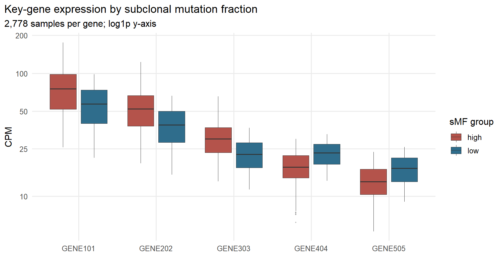
ImportantWhy DuckDB wins here
The two implementations compute an identical answer, and the gap comes from what never happens rather than from a faster aggregation.
Both return the same thing: one CPM value per gene per sample, 5 × 2,778 rows, enough to draw a distribution rather than just a mean.
The naive pipeline reads all 55.6 million count rows into R because it needs library sizes, then joins, then discards everything except five genes. Peak memory is set by the largest thing it ever held.
The DuckDB version expresses the same logic as one query, and the optimizer does two things a hand-written R script will not do for you. The library-size CTE streams over the counts and keeps only 2,778 sums. The main scan has the five-gene restriction pushed into it, so the file is read with a filter applied and 99.98% of the rows are discarded before they materialize anywhere.
That is the shape of problem a query engine handles best: a global computation over everything, feeding a question about almost nothing. It is also common in genomics: normalize on the whole matrix, then look at a pathway.
13 Scaling and memory pressure
13.1 Thread scaling
duck_sql <- function(source) sprintf("
  SELECT samplename, COUNT(*) AS n_snvs,
         COUNT(*) FILTER (cluster_id = mn) AS n_clonal,
         COUNT(*) - COUNT(*) FILTER (cluster_id = mn) AS n_subclonal,
         (COUNT(*) - COUNT(*) FILTER (cluster_id = mn))::DOUBLE / COUNT(*) AS sMF
  FROM (SELECT samplename, cluster_id,
               MIN(cluster_id) OVER (PARTITION BY samplename) mn FROM %s)
  GROUP BY ALL", source)

thread_grid <- sort(unique(c(1, 2, 4, 8, params$threads)))
sweep <- do.call(rbind, lapply(thread_grid, function(nthr) {
  # a heavier query, so thread differences are visible above the noise
  duck <- measure({
    cc <- dbConnect(duckdb(), config = list(threads = as.character(nthr)))
    on.exit(dbDisconnect(cc, shutdown = TRUE), add = TRUE)
    dbGetQuery(cc, sprintf(
      "SELECT COUNT(*) n FROM (SELECT * FROM read_parquet('%s') ORDER BY VAF, position)", PQ))
  }, sample_mem = FALSE)
  data.table::setDTthreads(nthr)
  dtt <- measure(dt[, .(n = .N, m = sum(cluster_id == min(cluster_id))), by = samplename],
                 sample_mem = FALSE)
  data.frame(threads = nthr, `DuckDB (sort 46M rows)` = duck$elapsed,
             `data.table (group)` = dtt$elapsed, check.names = FALSE)
}))
data.table::setDTthreads(params$threads)
kable(sweep, digits = 2, caption = "Scaling with thread count (seconds)")| threads | DuckDB (sort 46M rows) | data.table (group) |
|---|---|---|
| 1 | 0.85 | 0.47 |
| 2 | 0.85 | 0.45 |
| 4 | 0.86 | 0.42 |
| 8 | 0.84 | 0.54 |
sweep |>
  tidyr::pivot_longer(-threads, names_to = "engine", values_to = "elapsed") |>
  ggplot(aes(threads, elapsed, color = engine)) +
  geom_line(linewidth = .9) + geom_point(size = 2.6) +
  scale_x_continuous(breaks = thread_grid) +
  scale_color_manual(values = c("#2F6D8C", "#3E8E7E")) +
  theme(legend.position = "right") +
  labs(title = "Elapsed time vs thread count", x = "Threads", y = "Seconds")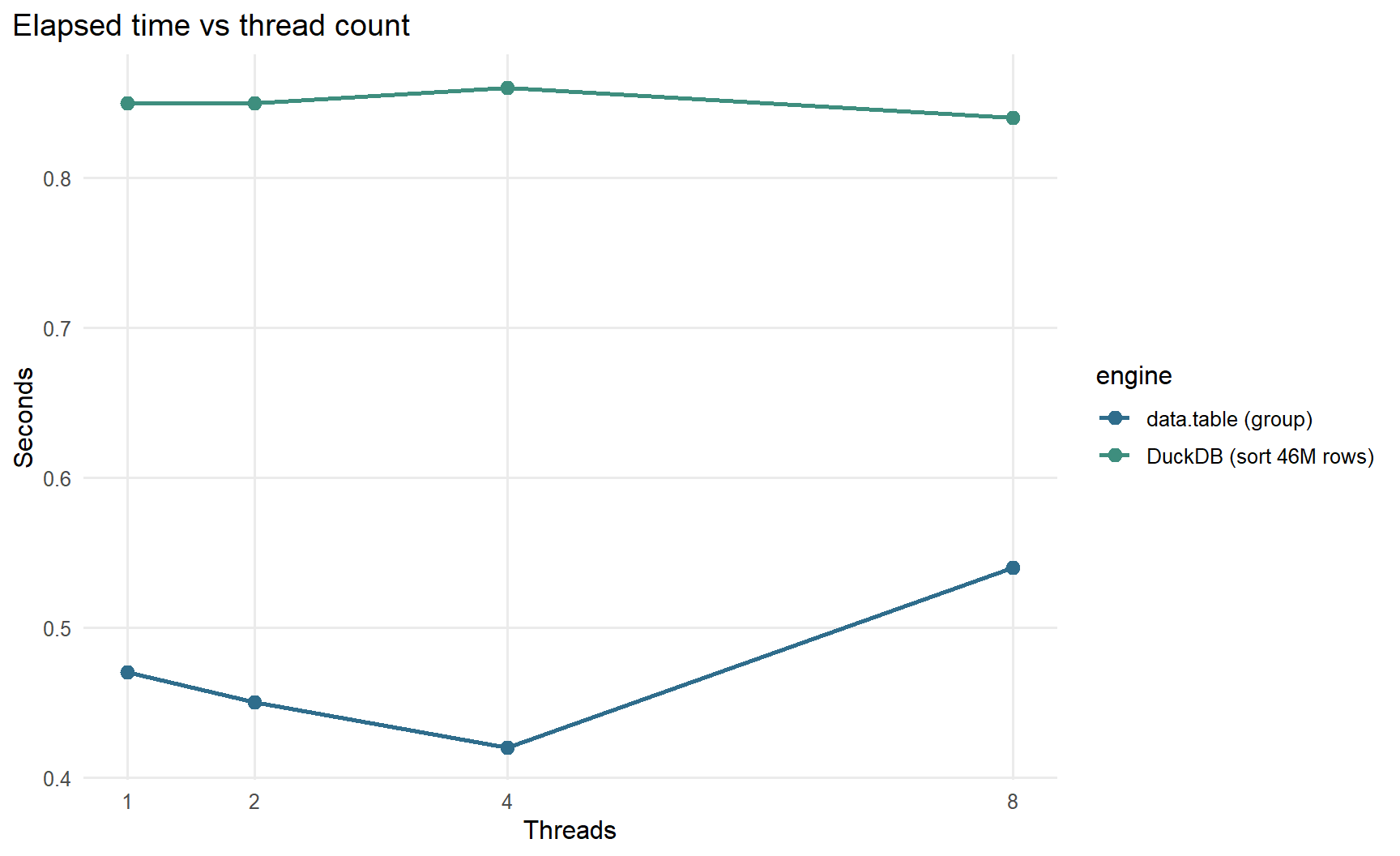
13.2 Working under a memory limit
The sMF query is a streaming aggregation and needs almost no working memory, so it is a poor stress test. Sorting every row is better, since a sort cannot emit its first row until it has seen the last.
sort_out <- tempfile(fileext = ".parquet")
lim_res <- do.call(rbind, lapply(c("1GB", "4GB", "24GB"), function(lim) {
  tdir <- file.path(tempdir(), paste0("spill_", gsub("[^A-Za-z0-9]", "", lim)))
  dir.create(tdir, showWarnings = FALSE)
  cc <- dbConnect(duckdb(), config = list(
    threads = as.character(params$threads), memory_limit = lim,
    temp_directory = gsub("\\\\", "/", tdir)))
  on.exit({ dbDisconnect(cc, shutdown = TRUE); unlink(tdir, recursive = TRUE) }, add = TRUE)
  unlink(sort_out)
  m <- measure(dbExecute(cc, sprintf(
    "COPY (SELECT * FROM read_parquet('%s') ORDER BY VAF, position) TO '%s' (FORMAT PARQUET)",
    PQ, gsub("\\\\", "/", sort_out))), sample_mem = TRUE)
  data.frame(memory_limit = lim, elapsed = m$elapsed, marginal_gb = m$delta_gb)
}))
unlink(sort_out)
kable(lim_res, digits = 2,
      caption = sprintf("A full %s-row sort under different DuckDB memory limits",
                        format(shape$rows, big.mark = ",")),
col.names = c("memory_limit", "Elapsed (s)", "Memory above baseline (GB)"))| memory_limit | Elapsed (s) | Memory above baseline (GB) |
|---|---|---|
| 1GB | 3.36 | 8.23 |
| 4GB | 3.39 | 8.90 |
| 24GB | 3.41 | 9.10 |
ImportantWhat this shows, and what it does not
The query completes at every limit, including one far below the size of the data. DuckDB sorted 46.1 million rows with its budget set to 1 GB. No in-memory method here can do that at all, since base R would need the whole table plus a sorted copy.
But memory_limit did not change runtime or process memory much. That is not a bug. DuckDB’s limit governs its buffer manager; the Parquet reader’s decompression buffers, the writer’s row-group buffers and query results all live outside it. Treat it as a guard against runaway intermediate state, not a hard cap on the process. DuckDB’s own guidance is 1 to 4 GB of limit per thread.
A caveat: I could not get this query to leave measurable evidence of spilling to disk. duckdb_memory() reports current state and DuckDB deletes its temp files the moment a query finishes, so a reading taken afterwards is always zero whether it spilled or not. The honest statement is that the query completed comfortably under a 1 GB budget, not that I proved how.
13.3 Scaling with data size
tmp_pq <- tempfile(fileext = ".parquet")
curve <- do.call(rbind, lapply(c(0.05, 0.15, 0.35, 0.65, 1.0), function(f) {
  cc <- dbConnect(duckdb(), config = list(threads = as.character(params$threads)))
  on.exit(dbDisconnect(cc, shutdown = TRUE), add = TRUE)
  n <- round(shape$rows * f)
  dbExecute(cc, sprintf("COPY (SELECT * FROM read_parquet('%s') LIMIT %d) TO '%s'
                         (FORMAT PARQUET, COMPRESSION ZSTD)", PQ, n, tmp_pq))
  a <- measure(dbGetQuery(cc, duck_sql(sprintf("read_parquet('%s')", tmp_pq))), sample_mem = FALSE)
  b <- measure(pl$scan_parquet(tmp_pq)$group_by("samplename")$agg(
                 pl$len()$alias("n_snvs"),
                 (pl$col("cluster_id") == pl$col("cluster_id")$min())$sum()$alias("n_clonal")
               )$collect(engine = "streaming"), sample_mem = FALSE)
  dd <- as.data.frame(arrow::read_parquet(tmp_pq))
  cl <- fmin(dd$cluster_id, g = dd$samplename, TRA = "replace")
  cc2 <- measure({ fnobs(dd$cluster_id, g = dd$samplename)
                   fsum(dd$cluster_id == cl, g = dd$samplename) }, sample_mem = FALSE)
  rm(dd); gc(FALSE)
  data.frame(rows = n, DuckDB = a$elapsed, polars = b$elapsed, collapse = cc2$elapsed)
}))
unlink(tmp_pq)
kable(curve, digits = 2, caption = "Elapsed seconds vs row count")| rows | DuckDB | polars | collapse |
|---|---|---|---|
| 2305779 | 0.01 | 0.03 | 0.00 |
| 6917338 | 0.03 | 0.10 | 0.05 |
| 16140456 | 0.06 | 0.20 | 0.09 |
| 29975132 | 0.10 | 0.38 | 0.18 |
| 46115588 | 0.14 | 0.59 | 0.26 |
curve |>
  tidyr::pivot_longer(-rows, names_to = "engine", values_to = "elapsed") |>
  ggplot(aes(rows, elapsed, color = engine)) +
  geom_line(linewidth = .9) + geom_point(size = 2.4) +
  scale_color_manual(values = c(DuckDB = "#2F6D8C", polars = "#B4534B", collapse = "#6AA84F")) +
  scale_x_continuous(labels = scales::label_number(scale_cut = scales::cut_short_scale())) +
  theme(legend.position = "right") +
  labs(title = "Scaling with row count", x = "Rows", y = "Seconds")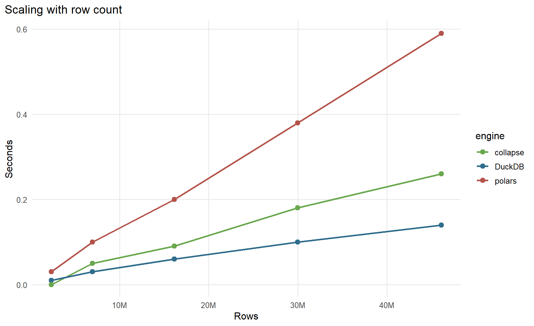
13.4 Writing results without materializing them
Every query so far returns a small table. When the output is also large, pulling it into R defeats the purpose. Polars can stream a query straight to a new Parquet file:
sink_out <- tempfile(fileext = ".parquet")
m_sink <- measure(
  pl$scan_parquet(PQ)$
    filter(pl$col("cluster_id") == 0L)$
    select("samplename", "chromosome", "position", "VAF")$
    sink_parquet(sink_out), sample_mem = TRUE)
cat(sprintf("streamed %.2f GB in %.1fs, peak RSS %.2f GB\n",
            file.info(sink_out)$size/GB, m_sink$elapsed, m_sink$peak_gb))
streamed 0.51 GB in 0.5s, peak RSS 13.89 GBunlink(sink_out)DuckDB’s equivalent is COPY (...) TO 'out.parquet' (FORMAT PARQUET, COMPRESSION ZSTD), which likewise never routes the data through R.
14 The tools, one at a time
Benchmarks rank things on one axis. Choosing a tool means weighing several. Here is an honest assessment of each.
14.1 Base R
Good at: being there. No dependencies, no installation, stable for decades, and every R user can read it.
Bad at: this. aggregate() was designed when datasets were thousands of rows, and it builds large per-group intermediates. It is also the only option here with no answer at all when data exceeds memory.
Use it when the data is small, the code must run anywhere with zero setup, or the operation is genuinely one-off. Do not reach for it to process tens of millions of rows.
14.2 dplyr
Good at: readability and ubiquity. group_by/summarize is the clearest expression of intent in this document, it composes well, and the entire tidyverse ecosystem plugs into it. .by = gives per-operation grouping without the group_by/ungroup dance and skips the sort.
Bad at: memory. Everything must be an R object first, and dplyr is not the fastest way to operate on those objects once they are.
Use it when clarity matters more than speed and the data fits comfortably, which is most of the time. And when it stops fitting, see duckplyr below, because you may not have to rewrite anything.
14.3 data.table
Good at: raw in-memory speed with a mature, stable API. Modify-by-reference (:=) avoids copies, fread is still among the fastest CSV parsers in any language, and the [i, j, by] form is extremely expressive once it clicks.
Bad at: approachability, since the syntax is genuinely a second language, and it is still fundamentally in-memory. Note that it had the highest peak memory of any method in Section 7, because converting from Arrow makes a copy.
Use it when your data fits in RAM, you are doing heavy in-memory manipulation, and your team already knows it. It remains an excellent choice and needs no apology.
14.4 collapse
Good at: speed-per-unit-of-rewriting. It provides C/C++ implementations of grouped statistics that keep base R’s data structures: no new frontend, no lazy frames, just faster versions of things you already do. TRA = "replace" broadcasting a grouped statistic back over rows is exactly the awkward step in our task.
Bad at: discoverability. The function names (fmin, fnobs, fsum, GRPN) are their own vocabulary, and, like everything above, it is in-memory only.
Use it when you have data in memory and want it faster without adopting a new paradigm. It is the most under-used package in this document.
14.5 Arrow
Good at: being the substrate. Arrow is the in-memory columnar format that Polars, DuckDB and modern R all speak, which is why data moves between them cheaply. The R package also gives you open_dataset() for multi-file and larger-than-memory data, excellent Parquet I/O, and dplyr verbs via the Acero engine.
Bad at: being a complete query engine. Acero does not support windowed mutate(), which is why our implementation needs a two-stage reformulation. You will hit its edges sooner than DuckDB’s or Polars’.
Use it when you need format conversion, Parquet reading and writing, or dataset discovery. Think of it as the plumbing rather than the destination.
14.6 DuckDB
Good at: nearly everything measured here. It was the fastest and lightest method in Section 7, queries Parquet on disk without importing it, spills to disk when it must, and speaks SQL, a language your collaborators, your database and your future self already know. Its dialect is unusually pleasant (GROUP BY ALL, SELECT * EXCLUDE, COUNT(*) FILTER (...), QUALIFY).
Bad at: nothing serious for this workload. The honest costs are that you must write SQL, which not every R user wants; that SQL is stricter than R in places that surprise people; and that results still have to cross into R eventually, which costs time proportional to result size.
Use it when the data is larger than memory, when you want one engine that handles files, databases and in-memory frames alike, or when SQL is a shared language on your team. It is the default recommendation of this document.
14.7 duckplyr
Good at: removing the choice above. It drives DuckDB’s relational API in-process with dplyr’s syntax and dplyr’s semantics, data frame in and data frame out, and falls back to dplyr for anything DuckDB cannot express, so it never simply fails.
Bad at: hiding what it is doing. That fallback is the whole point and also the main hazard: a pipeline can silently stop using DuckDB and become slow. Two concepts control this. Prudence governs automatic materialization, and "stingy" never materializes and turns a silent fallback into a visible error, which is what you want while developing. Fallback logging tells you after the fact:
duckplyr::fallback_sitrep()Use it when you have existing dplyr code and want it to scale without a rewrite. That is its entire premise and it delivers.
14.8 Polars
Good at: being a fast, coherent DataFrame library with a real query optimizer. Lazy mode plus scan_parquet() gives projection and predicate pushdown into the file; the streaming engine processes in batches rather than requiring everything at once; sink_parquet() writes results without materializing them. It was a close second to DuckDB throughout.
Bad at: stability and ergonomics in R. The R bindings are not on CRAN, so you install from R-multiverse, and the API was rewritten wholesale, so most Polars material you find online is for a version that no longer exists. The $-chained method syntax is also un-idiomatic in R.
Use it when you prefer a DataFrame API to SQL, you are already using Polars in Python and want consistency, or you need its streaming/sink capabilities. Use tidypolars if you want the engine with dplyr syntax, though note it errors on untranslated functions rather than falling back, the opposite trade-off from duckplyr.
WarningPolars gotchas
pl$DataFrame(df)does not do what you expect. It silently wraps a data frame into a single struct column instead of erroring. Useas_polars_df()/as_polars_lf().$collect(streaming = TRUE)is gone; it is$collect(engine = "streaming").- Vectors must be spliced into dynamic dots:
pl$col(!!!c("a","b")), notpl$col(c("a","b")). $count()ignores nulls;$len()does not.pl$len()is theCOUNT(*)you almost always want in$agg().POLARS_MAX_THREADSis locked when the package loads. Set it first.
Demonstrating the pl$DataFrame() trap
tiny <- head(d, 3)
cat("as_polars_df() columns:\n"); print(as_polars_df(tiny)$columns)
as_polars_df() columns: [1] "samplename" "chromosome" "position" "alt_count"
[5] "ref_count" "VAF" "cluster_id" "Subclonality"
[9] "purity" "major_cn" "minor_cn" "total_cn"
[13] "b_i^V" "CP_unpenalized" "CCF_unpenalized"Demonstrating the pl$DataFrame() trap
cat("\npl$DataFrame() columns:\n"); print(pl$DataFrame(tiny)$columns)
pl$DataFrame() columns:[1] ""15 Choosing
flowchart TD
    A[Does the data fit in RAM<br/>with room to spare?] -->|Yes| B[Do you need it faster?]
    A -->|No, or only just| C[Do you want SQL<br/>or a DataFrame API?]
    B -->|No| D[dplyr<br/>clarity wins]
    B -->|Yes, minimal rewrite| E[collapse]
    B -->|Yes, and I know it| F[data.table]
    C -->|SQL| G[DuckDB]
    C -->|Keep my dplyr code| H[duckplyr]
    C -->|DataFrame API| I[Polars<br/>scan + streaming]
    G --> J{Query the same data<br/>many times?}
    J -->|Yes| K[Import to .duckdb]
    J -->|No, or shared| L[Query Parquet directly]
15.1 Recommendations
Change your storage format before you change your library. Converting text to Parquet costs one line and buys most of the benefit available. Nothing else here has that ratio.
If the data does not fit in memory, use DuckDB. It was fastest and lightest, queries files in place, handles data larger than RAM, and SQL is a transferable skill. Reach for Polars instead if you prefer a DataFrame API or already use it in Python.
If you have dplyr code that has outgrown memory, use duckplyr before rewriting anything. Develop with prudence = "stingy" so fallbacks surface as errors rather than mysterious slowness.
If the data fits and you want it faster, reach for collapse first. It is the smallest change for the largest gain. data.table is excellent and worth it if you already know it or are doing heavy in-memory work.
Partition only on columns you filter by, and not too finely. The wrong partition key makes everything slower and bigger, as Section 6 measures.
Measure memory from outside R. Any R-level profiler will tell you DuckDB and Polars use no memory, which is wrong in a way that will mislead you badly.
15.2 Gotchas worth writing down
| Trap | Symptom | Fix |
|---|---|---|
profmem on DuckDB/Polars |
Engine “uses no memory” | Sample process RSS (Section 3) |
| Benchmarking in one session | In-memory tools look free | Cold start, fresh process (Section 3.2) |
| Timing a lazy pipeline | Impossibly fast | End in collect() |
Timing vroom() |
Impossibly fast, index only | altrep = FALSE |
pl$DataFrame(df) |
Missing-column errors | as_polars_df(df) |
$collect(streaming = TRUE) |
`...` must be empty |
$collect(engine = "streaming") |
pl$col(c("a","b")) |
Invalid input | pl$col(!!!c("a","b")) |
POLARS_MAX_THREADS set late |
Thread cap ignored | Set before library(polars) |
| Nested aggregate in SQL | aggregate function calls cannot be nested |
Two-stage group, then regroup |
| Silent duckplyr fallback | Unexpectedly slow | fallback_sitrep(), prudence = "stingy" |
| Over-partitioning | Everything slower and bigger | Partition on filtered columns only |
CAST(dbl AS INT) across engines |
DuckDB rounds, Polars truncates, a silent 1-base shift | Use an explicit FLOOR/ROUND everywhere |
| Polars join key type mismatch | datatypes of join keys don't match |
Cast both sides; Polars will not coerce |
| Assuming the purpose-built verb is fastest | Polars join_where slower than join+filter |
Measure both formulations |
LIMIT n with no ORDER BY |
Different rows on each engine/run | Never use it to build a comparable subset |
stats::reshape() on a big frame |
Minutes where seconds are expected | data.table::dcast() |
paste() key from a numeric column |
Silently loses rows to "1.3e+08" |
Pack into an integer, or sprintf("%.0f") |
| Range join as join-then-filter | Intermediate explodes (41.9 billion rows here) | Interval index, or a binned key |
| Globals inside a cold-start method | object not found in the child process |
Pass everything through arguments |
duckdb_memory() after a query |
Spill always reads 0 | Sample during execution |
Reporting user time |
Parallel engines look slow | Report elapsed |
| Cold vs warm page cache | Second engine always wins | Warm the file first, and say so |
16 Conclusion
Six workflows, each implemented several ways, each measured from a cold start with a harness that can see memory allocated outside R, and every implementation checked against a reference so that a fast wrong answer cannot win.
The dominant factor is whether the data ever becomes R objects. In workflows 1, 3, 4 and 6 the engines that read Parquet and return only the answer beat the in-memory approaches by one to two orders of magnitude in time, and by more than that in memory. Base R’s problem in Workflow 1 is that the table had to be loaded at all. aggregate() being slow is secondary, and collapse does the same calculation on the same data frame far faster. Workflow 6 is the sharpest version: a global normalization feeding a five-gene question, where the engine computes library sizes over 55.6 million rows without ever materializing them.
But the rule has real edges, and they are worth knowing. A range join (Workflow 2) is neither a scan nor a hash, so purpose-built interval structures match the column store on time, though DuckDB still wins on memory. Linear algebra (Workflow 5) has no SQL equivalent at all; both paths end in the same cor() call. And a query returning millions of rows (Workflow 3) spends a growing share of its time on the handover, narrowing the gap. The summary is push the work to the data, which is narrower than use DuckDB for everything.
You rarely have to choose between speed and familiarity any more. duckplyr runs dplyr code on DuckDB with the same semantics, tidypolars runs it on Polars, and duckdb_register() lets SQL query an R data frame with no copy. The practical advice for most people is therefore unglamorous: store it as Parquet, keep writing dplyr, and let duckplyr or DuckDB do the work.
And measure honestly. Building this document turned up a rounding difference between engines that silently shifted variants by one base, a join that quietly returned cross-chromosome matches, and a reshape that accounted for 90% of a runtime. None of those would have surfaced from timing alone. They surfaced because every result was compared against another. Every tool here is fast enough to look good under a benchmark designed to flatter it.
Session info
sessioninfo::session_info(pkgs = c("polars", "duckdb", "duckplyr", "arrow",
                                   "data.table", "dplyr", "collapse", "tidypolars"))
─ Session info ───────────────────────────────────────────────────────────────
setting value
version R version 4.5.1 (2025-06-13 ucrt)
os Windows 11 x64 (build 26200)
system x86_64, mingw32
ui RTerm
language (EN)
collate English_United States.utf8
ctype English_United States.utf8
tz America/New_York
date 2026-08-28
pandoc 3.8.3 @ C:\\Program Files\\RStudio\\resources\\app\\bin\\quarto\\bin\\tools/ (via rmarkdown)
quarto NA @ C:\\PROGRA~1\\RStudio\\RESOUR~1\\app\\bin\\quarto\\bin\\quarto.exe
─ Packages ───────────────────────────────────────────────────────────────────
package * version date (UTC) lib source
arrow * 25.0.0 2026-07-16 [1] CRAN (R 4.5.3)
assertthat 0.2.1 2019-03-21 [1] CRAN (R 4.5.3)
bit 4.6.0 2025-03-06 [1] CRAN (R 4.5.1)
bit64 4.6.0-1 2025-01-16 [1] CRAN (R 4.5.1)
cachem 1.1.0 2024-05-16 [1] CRAN (R 4.5.1)
cli 3.6.5 2025-04-23 [1] CRAN (R 4.5.1)
collapse * 2.1.7 2026-05-19 [1] CRAN (R 4.5.3)
collections 0.3.12 2026-03-22 [1] CRAN (R 4.5.3)
cpp11 0.5.2 2025-03-03 [1] CRAN (R 4.5.1)
data.table * 1.17.8 2025-07-10 [1] CRAN (R 4.5.1)
DBI * 1.2.3 2024-06-02 [1] CRAN (R 4.5.1)
dplyr * 1.2.0 2026-02-03 [1] CRAN (R 4.5.2)
duckdb * 1.5.5 2026-07-25 [1] CRAN (R 4.5.3)
duckplyr * 1.2.1 2026-03-10 [1] CRAN (R 4.5.3)
fastmap 1.2.0 2024-05-15 [1] CRAN (R 4.5.1)
generics 0.1.4 2025-05-09 [1] CRAN (R 4.5.1)
glue 1.8.0 2024-09-30 [1] CRAN (R 4.5.2)
jsonlite 2.0.0 2025-03-27 [1] CRAN (R 4.5.1)
lifecycle 1.0.5 2026-01-08 [1] CRAN (R 4.5.2)
magrittr 2.0.4 2025-09-12 [1] CRAN (R 4.5.1)
memoise 2.0.1 2021-11-26 [1] CRAN (R 4.5.1)
pillar 1.11.1 2025-09-17 [1] CRAN (R 4.5.1)
pkgconfig 2.0.3 2019-09-22 [1] CRAN (R 4.5.1)
polars * 1.13.0 2026-07-04 [1] https://r-multiverse.r-universe.dev (R 4.5.3)
purrr 1.2.1 2026-01-09 [1] CRAN (R 4.5.2)
R6 2.6.1 2025-02-15 [1] CRAN (R 4.5.1)
Rcpp 1.1.2 2026-07-05 [1] CRAN (R 4.5.3)
rlang 1.3.0 2026-07-05 [1] CRAN (R 4.5.3)
S7 0.2.2 2026-04-20 [1] https://r-multiverse.r-universe.dev (R 4.5.3)
stringi 1.8.7 2025-03-27 [1] CRAN (R 4.5.0)
stringr 1.6.0 2025-11-04 [1] CRAN (R 4.5.2)
tibble 3.3.1 2026-01-11 [1] CRAN (R 4.5.2)
tidypolars * 0.19.0 2026-07-04 [1] https://r-multiverse.r-universe.dev (R 4.5.3)
tidyr 1.3.2 2025-12-19 [1] CRAN (R 4.5.2)
tidyselect 1.2.1 2024-03-11 [1] CRAN (R 4.5.1)
utf8 1.2.6 2025-06-08 [1] CRAN (R 4.5.1)
vctrs 0.7.1 2026-01-23 [1] CRAN (R 4.5.2)
withr 3.0.2 2024-10-28 [1] CRAN (R 4.5.1)
[1] C:/Users/Matthew/AppData/Local/R/win-library/4.5
[2] C:/Program Files/R/R-4.5.1/library
* ── Packages attached to the search path.
──────────────────────────────────────────────────────────────────────────────