Tools for working with large data in R

Base R, data.table, Arrow, DuckDB and Polars — benchmarked honestly

1 Introduction

When a dataset stops fitting comfortably in memory, the tool you reach for matters more than the code you write with it. This workshop works through one realistic genomics task on a 46-million-row table, implementing it about twenty different ways — from read.table() and aggregate() through to Polars’ streaming engine and DuckDB’s out-of-core SQL — and measures what each one actually costs in time and memory.

Two things distinguish this version of the tutorial from the one I first wrote in 2024:

1. The benchmarking is honest. The original measured memory with profmem, which only sees allocations made through R’s own allocator. DuckDB, Polars and Arrow allocate in C++/Rust heaps, so they reported approximately zero memory used — which flattered them enormously and was simply wrong. Section 4 explains the problem and replaces it with a sampled peak-RSS measurement.
2. The tools have moved. Polars had a complete API rewrite, DuckDB reached 1.0 and then 1.5, and duckplyr went from “doesn’t quite work” to a genuine drop-in for dplyr. Code from the 2024 edition does not all still run. Section 2 lists the breaking changes.

TipHow to run this document

The params block at the top of the source controls cost:

• scale: "demo" builds a 200-sample subset and renders in a few minutes. Use this while you are editing.
• scale: "full" uses all 46M rows. Expect a long render, mostly because of read.table().
• run_read_table: false skips the single slowest chunk.
• threads caps every engine to the same number of cores. Comparing 16-thread DuckDB against single-threaded base R is not a benchmark, it is a press release.

2 What changed since 2024

If you are updating your own materials, these are the changes that will actually break code.

2.1 Polars: the 1.0 rewrite

r-polars was rewritten from scratch. The version here is 1.13.0, tracking Python Polars 1.42. Old code fails in ways that range from loud to dangerous:

2024 code	Status now	Replacement
pl$DataFrame(df)	Silently wrong	as_polars_df(df)
$to_data_frame()	Removed	as.data.frame()
$to_r(), $to_list()	Removed	as.vector(), as.list()
pl$dtypes$Float64	Removed	pl$Float64
$collect(streaming = TRUE)	Hard error	$collect(engine = "streaming")
pl$col(c("a","b"))	Error	pl$col(!!!c("a","b"))
$profile()	Being retired	$explain() + bench::mark()

WarningThe dangerous one

pl$DataFrame(df) no longer errors on a data frame — it silently wraps the whole thing into a single struct column. Every downstream pl$col("samplename") then fails with a confusing message about a missing column, and if your pipeline happens not to reference a column by name you can get a plausible-looking wrong answer. We demonstrate this in Section 7.2.

Use as_polars_df() / as_polars_lf() instead. Always.

Polars is not on CRAN (archived in 2023 over Rust vendoring policy, never restored). Install it from R-multiverse:

Sys.setenv(NOT_CRAN = "true")   # use the pre-built Rust binary instead of compiling
install.packages("polars", repos = "https://community.r-multiverse.org")
install.packages("tidypolars", repos = "https://community.r-multiverse.org")

If you have old code you cannot rewrite today, the pre-rewrite API is published separately as polars0 and installs alongside the new one.

2.2 DuckDB: 1.0 → 1.5

DuckDB hit 1.0 in June 2024 with a storage format guarantee, and is now at 1.5.5. Highlights that matter here: an external file cache (1.3) that makes repeated remote Parquet scans dramatically faster; a rewritten k-way merge sort (1.4 LTS) that behaves far better out-of-core; MERGE INTO, database encryption and Iceberg writes (1.4); and the VARIANT type plus core GEOMETRY (1.5).

Day to day the friendly SQL dialect matters more than any of that — GROUP BY ALL, SELECT * EXCLUDE (...), QUALIFY, COUNT(*) FILTER (...) and FROM-first queries all remove boilerplate, and we use them throughout.

2.3 duckplyr became real

The 2024 edition of this tutorial contained the line “I have found it to not behave as expected for complicated queries.” That is no longer a fair assessment. duckplyr 1.2.1 is part of the tidyverse and is a genuine drop-in: same syntax and same semantics as dplyr, with automatic fallback to dplyr for anything DuckDB cannot do. Section 7.3.3 covers its two new concepts, prudence and fallback.

3 Setup

ImportantThread caps must come first

POLARS_MAX_THREADS is read when the Rust thread pool initializes and cannot be changed after library(polars). It has to be set before the package is loaded — so this is the first executable line in the document.

Sys.setenv(POLARS_MAX_THREADS = as.character(params$threads))
Sys.setenv(RETICULATE_PYTHON = normalizePath(".venv/Scripts/python.exe", mustWork = FALSE))

suppressPackageStartupMessages({
  library(dplyr);  library(ggplot2); library(data.table); library(collapse)
  library(arrow);  library(DBI);     library(duckdb);     library(dbplyr)
  library(duckplyr, warn.conflicts = FALSE)
  library(polars); library(tidypolars)
  library(dtplyr); library(bench);   library(knitr)
})
source("bench_helpers.R")   # measure(), run_suite(), canon() -- see @sec-bench

# Apply the same thread cap everywhere we can
data.table::setDTthreads(params$threads)
arrow::set_cpu_count(params$threads)
options(duckdb.threads = params$threads)

theme_set(theme_minimal(base_size = 12) +
          theme(legend.position = "none",
                panel.grid.minor = element_blank(),
                plot.title.position = "plot"))
fam_pal <- c("base R" = "#7B6B8F", "tidyverse" = "#4C6EA8", "data.table" = "#3E8E7E",
             "collapse" = "#6AA84F", "arrow" = "#C0873F", "polars" = "#B4534B",
             "DuckDB" = "#2F6D8C", "other" = "#8A8A8A")

hw <- hardware_info()
tibble::tibble(
  Item = c("OS", "R", "CPU (logical / physical)", "RAM", "Thread cap for benchmarks"),
  Value = c(hw$os, hw$r_version,
            paste(hw$logical_cpu, "/", hw$phys_cpu),
            sprintf("%.1f GB", hw$ram_gb),
            as.character(params$threads))
) |> kable()

Item	Value
OS	Windows 10 x64
R	4.5.1
CPU (logical / physical)	16 / 8
RAM	93.6 GB
Thread cap for benchmarks	8

pkgs <- c("polars", "tidypolars", "duckdb", "duckplyr", "arrow", "data.table",
          "dplyr", "dtplyr", "collapse", "dbplyr", "bench", "fst", "qs2", "nanoarrow")
tibble::tibble(Package = pkgs, Version = vapply(pkgs, pkg_ver, character(1))) |>
  kable(caption = "Package versions used for these results")

Package versions used for these results

Package	Version
polars	1.13.0
tidypolars	0.19.0
duckdb	1.5.5
duckplyr	1.2.1
arrow	25.0.0
data.table	1.17.8
dplyr	1.2.0
dtplyr	1.3.3
collapse	2.1.7
dbplyr	2.5.1
bench	1.1.4
fst	0.9.8
qs2	0.2.2
nanoarrow	0.8.0.1

3.1 The dataset

The example is aggregated CliPP output for all PCAWG samples. To avoid any issues with protected data, the file below has the same shape — same row count, same sample count, same column structure — as the real CliPP output, but the values are randomly generated.

FULL_TSV <- "fake_pcawg_all.tsv"
FULL_PQ  <- "fake_pcawg_all.parquet"

con0 <- dbConnect(duckdb())
if (identical(params$scale, "demo")) {
  # A 200-sample subset: same structure, ~7% of the rows, renders quickly.
  PQ <- "dev_subsample.parquet"
  if (!file.exists(PQ)) {
    dbExecute(con0, sprintf("
      COPY (SELECT * FROM read_parquet('%s') WHERE samplename IN (
              SELECT samplename FROM read_parquet('%s')
              GROUP BY samplename ORDER BY samplename LIMIT 200))
      TO '%s' (FORMAT PARQUET, COMPRESSION ZSTD)", FULL_PQ, FULL_PQ, PQ))
  }
  TSV <- NA_character_   # the TSV read benchmarks only make sense at full scale
  # The shipped .duckdb file holds the full table; build a matching subset one so
  # that every method in @sec-compute is answering the same question.
  DB <- "dev_subsample.duckdb"
  if (!file.exists(DB)) {
    cdb <- dbConnect(duckdb(), DB)
    dbExecute(cdb, sprintf("CREATE TABLE pcawg_all AS SELECT * FROM read_parquet('%s')", PQ))
    dbDisconnect(cdb, shutdown = TRUE)
  }
} else {
  PQ  <- FULL_PQ
  TSV <- FULL_TSV
  DB  <- "pcawg_data.duckdb"
}

shape <- dbGetQuery(con0, sprintf(
  "SELECT COUNT(*) AS rows, COUNT(DISTINCT samplename) AS samples FROM read_parquet('%s')", PQ))
schema_tbl <- dbGetQuery(con0, sprintf(
  "SELECT column_name, column_type FROM (DESCRIBE SELECT * FROM read_parquet('%s'))", PQ))
dbDisconnect(con0, shutdown = TRUE)

cat(sprintf("scale = %s\n%s rows x %d columns, %s samples\n",
            params$scale, format(shape$rows, big.mark = ","),
            nrow(schema_tbl), format(shape$samples, big.mark = ",")))

scale = full
46,115,588 rows x 15 columns, 2,778 samples

kable(schema_tbl, caption = "Schema")

Schema

column_name	column_type
samplename	VARCHAR
chromosome	INTEGER
position	DOUBLE
alt_count	INTEGER
ref_count	INTEGER
VAF	DOUBLE
cluster_id	INTEGER
Subclonality	VARCHAR
purity	DOUBLE
major_cn	INTEGER
minor_cn	INTEGER
total_cn	INTEGER
b_i^V	INTEGER
CP_unpenalized	DOUBLE
CCF_unpenalized	DOUBLE

3.2 The task: subclonal mutation fraction (sMF)

For each sample we want the fraction of mutations that are subclonal. Every mutation is assigned to a cluster; the cluster with the lowest cluster_id is the clonal cluster, and everything else is subclonal.

\[ \text{sMF}_s = \frac{n^{\text{subclonal}}_s}{n^{\text{SNV}}_s} = 1 - \frac{\#\{i \in s : \texttt{cluster\_id}_i = \min_{j \in s} \texttt{cluster\_id}_j\}}{\#\{i \in s\}} \]

It is deliberately unglamorous: a grouped minimum, a comparison against it, and two grouped counts. What makes it interesting as a benchmark is that the grouped minimum has to be broadcast back to every row before the counting happens, so an engine either needs a window function, a join, or two passes over the data. That is exactly the shape of computation where engines diverge.

Every implementation below must return one row per sample with columns samplename, n_snvs, n_clonal, n_subclonal, sMF.

4 How to benchmark this honestly

Before any numbers, the measurement. This section exists because the 2024 version of this tutorial got it wrong, and the way it got it wrong is the single most common mistake in R benchmarking blog posts.

4.1 The bug: R’s profiler cannot see foreign memory

The original harness was built on profmem:

mem_profile   <- profmem::profmem(expr)
total_mem_gb  <- sum(mem_profile$bytes) / 1024^3
peak_mem_gb   <- max(mem_profile$bytes) / 1024^3   # <- not a peak

There are two independent problems.

profmem only sees R’s allocator. It hooks Rprofmem, which records allocations made through R’s memory manager. DuckDB, Polars and Arrow are compiled C++/Rust libraries that call malloc themselves. To profmem they are invisible. The same blind spot affects bench::mark()’s mem_alloc column and the peakRAM package — all three report zero for a gigabyte allocated in C++.

max(bytes) is not a peak. It is the size of the largest single allocation. A workload that allocates 1 GB five times over shows a “peak” of 1 GB whether those allocations coexist or not. And sum(bytes) is worse — it is total allocation churn, which over-reports badly whenever R copies a vector.

Here is the discrepancy on real data. Both columns describe the same DuckDB query:

con <- dbConnect(duckdb())
q_read <- sprintf("SELECT * FROM read_parquet('%s')", PQ)

pm  <- profmem::profmem({ x <- dbGetQuery(con, q_read); nrow(x) }); rm(x); gc(FALSE)

          used (Mb) gc trigger   (Mb)  max used   (Mb)
Ncells 1859385 99.4    3716928  198.6   2358165  126.0
Vcells 3238973 24.8  447490818 3414.1 510590528 3895.5

rss <- measure({ x <- dbGetQuery(con, q_read); nrow(x) });          rm(x); gc(FALSE)

          used  (Mb) gc trigger   (Mb)  max used   (Mb)
Ncells 1893029 101.1    3716928  198.6   1948697  104.1
Vcells 3305162  25.3  537132556 4098.0 510634516 3895.9

dbDisconnect(con, shutdown = TRUE)

tibble::tibble(
  Measurement = c("profmem: sum(bytes)", "profmem: max(bytes)  [the old 'peak']",
                  "Sampled peak RSS  [reality]"),
  GB = c(sum(pm$bytes, na.rm = TRUE)/GB, max(pm$bytes, na.rm = TRUE)/GB, rss$delta_gb)
) |> kable(digits = 3, caption = "Same DuckDB query, three 'memory' numbers")

Same DuckDB query, three ‘memory’ numbers

Measurement	GB
profmem: sum(bytes)	3.779
profmem: max(bytes) [the old ‘peak’]	0.344
Sampled peak RSS [reality]	9.779

The R-level profiler misses essentially all of it, because essentially all of it was allocated by DuckDB.

4.2 The fix: sample the operating system’s view

The only reliable measurement is the resident set size (RSS) of the whole R process, sampled from outside while the expression runs. Since R is blocked during the call, the sampler has to live in a separate process. bench_helpers.R implements this:

measure(expr)   # -> elapsed, cpu, peak_gb, delta_gb, r_alloc_gb, n_samples

A background R process polls this process’s RSS every 50 ms and republishes its running maximum to a file, so we can kill it at any point and still recover the value. Two details matter:

• Do not poll ps::ps_children() — it costs ~850 ms per call on Windows, which would leave you with one sample per run. It is also unnecessary: DuckDB, Polars and Arrow are loaded into the R process, so R’s own RSS already includes them. You would only need child accounting if you shelled out to a separate duckdb.exe.
• Peak working set cannot be reset on Windows. ps_memory_info()$peak_wset is monotonic for the life of the process and no API resets it, so it is only usable for the first measurement in a session. Sampling sidesteps this entirely.

NoteRead n_samples before you trust a memory number

At a 50 ms sampling interval, a 30 ms workload gets one or two samples and its peak is basically noise — it can even come out slightly negative, since the baseline is taken after a gc() that may have released more than the workload allocates. Memory figures below are meaningful for the multi-second workloads and should be ignored for the fast ones. Time is measured exactly regardless.

4.3 Three more things that quietly ruin benchmarks

Wall time and CPU time are different questions. system.time() reports user as CPU summed across all threads, so a well-parallelized engine shows user far greater than elapsed. Only elapsed is comparable across engines — reporting user would rank the fastest engine last. The ratio is informative in its own right, so the tables below carry a parallelism column (cpu / elapsed).

The page cache. After one read, a file sits in the OS cache and every subsequent read is warm — often several times faster. Whichever engine you benchmark second wins. On Windows you cannot drop the cache from R (there is no /proc/sys/vm/drop_caches; you would need Sysinternals RAMMap or EmptyStandbyList.exe, both external and both needing admin). The reproducible alternative is to standardize on warm: read the file once before timing anything, and say so.

warm <- function(path) if (!is.na(path) && file.exists(path))
  invisible(readBin(path, "raw", n = file.size(path)))
warm(PQ)
gc(full = TRUE)

            used   (Mb) gc trigger   (Mb)  max used   (Mb)
Ncells   1892588  101.1    3716928  198.6   1973185  105.4
Vcells 151089593 1152.8  429706045 3278.4 510634516 3895.9

The lazy-evaluation trap. Polars scan_*, DuckDB dbSendQuery, arrow::open_dataset and dbplyr’s tbl() all return immediately without doing any work. Time one of those without materializing and you have benchmarked query planning — microseconds — and will conclude Polars is a thousand times faster than it is. Every lazy pipeline below ends in collect(), and run_suite() checks the returned result, so a pipeline that did nothing cannot pass.

4.4 The correctness check nobody runs

A fast wrong answer is not a benchmark result. Engines differ in row order, in integer versus double types, and in tibble versus data.frame versus data.table containers, so results need canonicalizing before comparison. canon() does that, and run_suite() compares every method against the first one:

print(canon)

function (x, digits = 8) 
{
    if (inherits(x, "polars_data_frame") || inherits(x, "polars_lazy_frame")) {
        if (inherits(x, "polars_lazy_frame")) 
            x <- x$collect()
        x <- as.data.frame(x)
    }
    x <- as.data.frame(x, stringsAsFactors = FALSE)
    keep <- c("samplename", "n_snvs", "n_clonal", "n_subclonal", 
        "sMF")
    stopifnot(all(keep %in% names(x)))
    x <- x[, keep, drop = FALSE]
    x$samplename <- as.character(x$samplename)
    x$n_snvs <- as.numeric(x$n_snvs)
    x$n_clonal <- as.numeric(x$n_clonal)
    x$n_subclonal <- as.numeric(x$n_subclonal)
    x$sMF <- round(as.numeric(x$sMF), digits)
    x <- x[order(x$samplename), , drop = FALSE]
    rownames(x) <- NULL
    x
}

Any method whose answer diverges is reported as MISMATCH rather than being quietly ranked. This caught two genuine bugs while updating this document, both described in Section 7.

5 Part 1 — Storage formats

The single largest speedup available is usually not a faster library. It is not storing 6.5 GB of numbers as text.

fmt_dir <- "format_bakeoff"; dir.create(fmt_dir, showWarnings = FALSE)
p <- function(f) file.path(fmt_dir, f)

d_mem <- as.data.frame(arrow::read_parquet(PQ))   # one in-memory copy to write from

write_specs <- list(
  list(name = "TSV (text)",          file = p("d.tsv"), needs = "data.table",
       write = function() data.table::fwrite(d_mem, p("d.tsv"), sep = "\t")),
  list(name = "TSV + gzip",          file = p("d.tsv.gz"), needs = "data.table",
       write = function() data.table::fwrite(d_mem, p("d.tsv.gz"), sep = "\t", compress = "gzip")),
  list(name = "Parquet (snappy)",    file = p("d_snappy.parquet"), needs = "arrow",
       write = function() arrow::write_parquet(d_mem, p("d_snappy.parquet"), compression = "snappy")),
  list(name = "Parquet (zstd)",      file = p("d_zstd.parquet"), needs = "arrow",
       write = function() arrow::write_parquet(d_mem, p("d_zstd.parquet"), compression = "zstd")),
  list(name = "Arrow IPC / feather", file = p("d.arrow"), needs = "arrow",
       write = function() arrow::write_feather(d_mem, p("d.arrow"), compression = "lz4")),
  list(name = "fst",                 file = p("d.fst"), needs = "fst",
       write = function() fst::write_fst(d_mem, p("d.fst"), compress = 50)),
  list(name = "qs2",                 file = p("d.qs2"), needs = "qs2",
       write = function() qs2::qs_save(d_mem, p("d.qs2")))
)
# Drop any format whose package will not load on this machine, rather than
# aborting the whole document.
write_specs <- Filter(function(s) all(vapply(s$needs, have_pkg, logical(1))), write_specs)

fmt_rows <- lapply(write_specs, function(s) {
  m <- measure(s$write(), sample_mem = FALSE)
  data.frame(format = s$name, write_s = m$elapsed,
             size_gb = file.info(s$file)$size / GB, stringsAsFactors = FALSE)
})
fmt <- do.call(rbind, fmt_rows)
fmt$vs_tsv <- fmt$size_gb[1] / fmt$size_gb
rm(d_mem); gc(full = TRUE)

          used  (Mb) gc trigger   (Mb)  max used   (Mb)
Ncells 2048485 109.5    3716928  198.6   2068716  110.5
Vcells 3579853  27.4  978975288 7469.0 510947358 3898.3

kable(fmt, digits = 2, col.names = c("Format", "Write (s)", "Size (GB)", "x smaller than TSV"),
      caption = "Same data, seven encodings")

Same data, seven encodings

Format	Write (s)	Size (GB)	x smaller than TSV
TSV (text)	2.97	6.40	1.00
TSV + gzip	20.02	1.70	3.76
Parquet (snappy)	11.07	1.09	5.85
Parquet (zstd)	11.45	1.01	6.32
Arrow IPC / feather	5.13	1.92	3.34
fst	1.67	2.10	3.04
qs2	7.10	0.97	6.60

fmt |>
  transform(format = factor(format, levels = format[order(size_gb)])) |>
  ggplot(aes(size_gb, format, fill = size_gb)) +
  geom_col(width = .68) +
  geom_text(aes(label = sprintf("%.2f GB", size_gb)), hjust = -0.12, size = 3.6) +
  scale_fill_gradient(low = "#2F6D8C", high = "#B4534B") +
  scale_x_continuous(expand = expansion(mult = c(0, .18))) +
  labs(title = "File size by storage format", x = "GB on disk", y = NULL)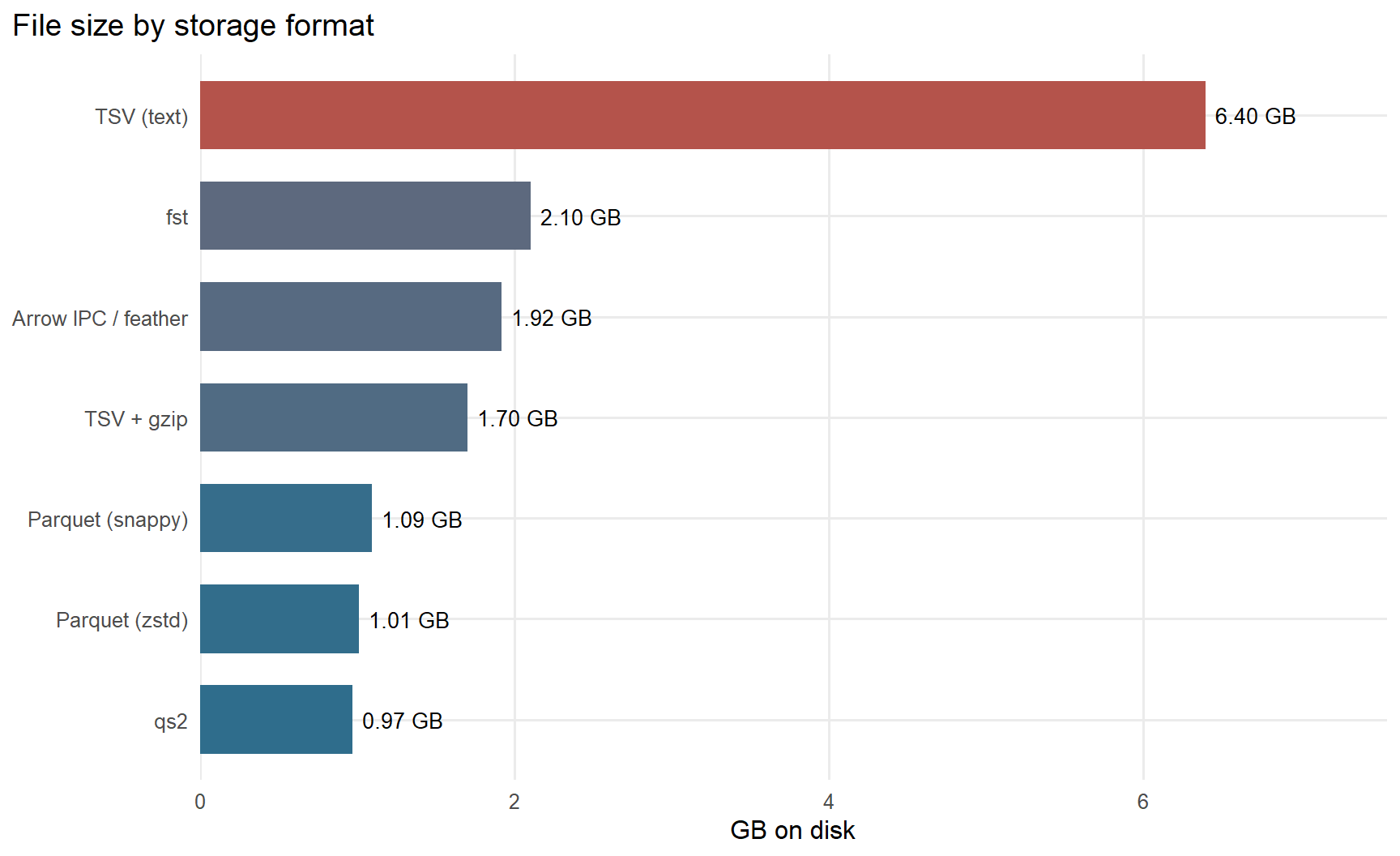

Figure 1: Storage cost of the same 46M-row table. Columnar formats win twice: smaller on disk, and only the columns you ask for get read.

5.1 What Parquet actually buys you

Parquet is a binary, columnar, compressed format. Data is stored column by column rather than row by row, in independently-compressed chunks called row groups (this file has 44 of them), each carrying min/max statistics for its columns.

That layout produces three distinct wins, and it is worth separating them because only the first is about file size:

1. Compression. Values within a column are homogeneous, so they compress far better than a row of mixed types. Snappy is fast to decompress; zstd is meaningfully smaller for a little more CPU and is the better default today.
2. Projection pushdown. Reading 2 of 15 columns reads roughly 2/15ths of the bytes. In a row-oriented format you must read every row in full and discard.
3. Predicate pushdown. Row-group statistics let a reader skip whole chunks that cannot contain matching rows, without decompressing them.

The last two are properties of the reader, not the file, which is why they show up in the Polars and DuckDB numbers and not in the base R ones. We measure them directly in Section 6.3.

The costs are real but narrow: Parquet is not human-readable, the overhead is not worth it for small data, and writes are slower than appending to a CSV. For a workshop dataset that is read many times and written once, that trade is overwhelmingly favorable.

5.2 .duckdb files versus Parquet

A .duckdb file is DuckDB’s own storage format. Compared with Parquet it trades portability for query speed: it carries indexes and zone maps, supports transactional updates, and DuckDB queries it faster than it queries Parquet. But only DuckDB reads it, and it is larger — 3.33 GB here against 1.10 GB for snappy Parquet.

Rule of thumb: Parquet for data you share or archive, .duckdb for a working set you query repeatedly. Since DuckDB 1.0 the storage format is stable across versions, so a .duckdb file is no longer a throwaway artifact.

6 Part 2 — Reading data

6.1 Reading text

This is the section that motivates everything else. read.table() on the full 6.5 GB TSV is the slowest thing in the document by a wide margin — it parses text in R, guesses types by scanning, and grows vectors as it goes.

text_methods <- list(
  bench_method("data.table::fread", "data.table",
               function() data.table::fread(TSV, nThread = params$threads),
               "parallel C parser"),
  bench_method("vroom (ALTREP, lazy)", "tidyverse",
               function() vroom::vroom(TSV, delim = "\t", show_col_types = FALSE,
                                       num_threads = params$threads),
               "builds an index only -- see callout"),
  bench_method("vroom (materialized)", "tidyverse",
               function() vroom::vroom(TSV, delim = "\t", show_col_types = FALSE,
                                       num_threads = params$threads, altrep = FALSE),
               "forced to read every column"),
  bench_method("readr::read_delim", "tidyverse",
               function() readr::read_delim(TSV, delim = "\t", show_col_types = FALSE,
                                            num_threads = params$threads),
               "second-gen tidyverse parser"),
  bench_method("polars scan_csv", "polars",
               function() pl$scan_csv(TSV, separator = "\t")$collect(engine = "streaming"),
               "Rust, multithreaded"),
  bench_method("DuckDB read_csv", "DuckDB",
               function() {
                 cc <- dbConnect(duckdb(), config = list(threads = as.character(params$threads)))
                 on.exit(dbDisconnect(cc, shutdown = TRUE), add = TRUE)
                 dbGetQuery(cc, sprintf("SELECT * FROM read_csv('%s', delim='\t', header=true)", TSV))
               }, "parallel CSV sniffer")
)
if (isTRUE(params$run_read_table)) {
  text_methods <- c(list(bench_method("base R read.table", "base R",
    function() utils::read.table(TSV, header = TRUE, sep = "\t", quote = "\""),
    "the 'don't' baseline")), text_methods)
}

read_res <- run_suite(text_methods, reference = NULL, sample_mem = TRUE)

read_res |>
  transform(GB_per_s = (file.size(TSV)/GB) / elapsed) |>
  subset(select = c(method, note, elapsed, peak_gb, parallelism, GB_per_s)) |>
  kable(digits = 2, caption = "Reading a 6.5 GB tab-separated file",
        col.names = c("Method", "Note", "Elapsed (s)", "Peak RSS (GB)", "CPU/wall", "GB/s"))

Table 1: Reading a 6.5 GB tab-separated file

Method	Note	Elapsed (s)	Peak RSS (GB)	CPU/wall	GB/s
base R read.table	the ‘don’t’ baseline	297.21	20.43	0.99	0.02
data.table::fread	parallel C parser	2.88	14.97	4.04	2.27
vroom (ALTREP, lazy)	builds an index only – see callout	3.36	17.29	7.42	1.94
vroom (materialized)	forced to read every column	13.00	21.88	4.61	0.50
readr::read_delim	second-gen tidyverse parser	13.05	21.87	4.62	0.50
polars scan_csv	Rust, multithreaded	4.20	19.13	3.61	1.55
DuckDB read_csv	parallel CSV sniffer	5.35	17.47	4.94	1.22

WarningThe two vroom rows are the lazy trap, live

vroom is deliberately lazy: by default it builds an index of where each field starts and returns immediately, materializing a column only when you touch it. The “ALTREP, lazy” row above therefore measures index construction, not reading, and it will look impossibly fast next to everything else.

That is not a criticism of vroom — deferring work you may never need is a genuinely good strategy, and if you only use three of fifteen columns you never pay for the other twelve. It is a criticism of benchmarking it naively. The “materialized” row passes altrep = FALSE to force a like-for-like comparison, and that is the number to read against fread and the others.

This is the same trap as timing a Polars scan_* without collect(), and it is easy to fall into precisely because the tool is behaving sensibly.

NoteWhy read.table() is so much slower

It is not merely that the parser is written in R. read.table() reads the file twice by default (once to infer types), builds every column as a growing R vector, and converts strings one at a time through R’s global string cache. fread and the Rust/C++ parsers memory-map the file, split it into chunks, and parse those chunks in parallel straight into typed buffers.

Note also the original 2024 tutorial’s call: read.table(file, sep = "\t") with no header = TRUE. That silently reads the header line as data and names the columns V1…V15, which is a good example of why the correctness check in Section 4 matters.

6.2 Reading binary formats

bin_methods <- list(
  bench_method("arrow::read_parquet", "arrow",
               function() as.data.frame(arrow::read_parquet(p("d_snappy.parquet"))), "snappy"),
  bench_method("arrow::read_parquet (zstd)", "arrow",
               function() as.data.frame(arrow::read_parquet(p("d_zstd.parquet"))), "zstd"),
  bench_method("polars read_parquet", "polars",
               function() as.data.frame(pl$read_parquet(p("d_snappy.parquet"))), "Rust reader"),
  bench_method("DuckDB -> data.frame", "DuckDB",
               function() {
                 cc <- dbConnect(duckdb(), config = list(threads = as.character(params$threads)))
                 on.exit(dbDisconnect(cc, shutdown = TRUE), add = TRUE)
                 dbGetQuery(cc, sprintf("SELECT * FROM read_parquet('%s')", p("d_snappy.parquet")))
               }, "via DBI"),
  bench_method("arrow::read_feather", "arrow",
               function() as.data.frame(arrow::read_feather(p("d.arrow"))), "Arrow IPC, lz4"),
  bench_method("fst::read_fst", "other",
               function() fst::read_fst(p("d.fst")), "R-specific, seekable", needs = "fst"),
  bench_method("qs2::qs_read", "other",
               function() qs2::qs_read(p("d.qs2")), "R serialization", needs = "qs2")
)
# only benchmark readers whose file actually got written above
bin_methods <- Filter(function(m) all(vapply(m$needs, have_pkg, logical(1))), bin_methods)
bin_res <- run_suite(bin_methods, reference = NULL, sample_mem = TRUE)
bin_res |>
  subset(select = c(method, note, elapsed, peak_gb, parallelism)) |>
  kable(digits = 2, caption = "Reading the same data from binary formats",
        col.names = c("Method", "Note", "Elapsed (s)", "Peak RSS (GB)", "CPU/wall"))

Reading the same data from binary formats

Method	Note	Elapsed (s)	Peak RSS (GB)	CPU/wall
arrow::read_parquet	snappy	3.73	12.35	1.00
arrow::read_parquet (zstd)	zstd	4.03	17.79	1.01
polars read_parquet	Rust reader	10.80	18.61	1.20
DuckDB -> data.frame	via DBI	3.63	20.19	2.61
arrow::read_feather	Arrow IPC, lz4	0.66	17.90	4.02
fst::read_fst	R-specific, seekable	3.11	13.95	1.70
qs2::qs_read	R serialization	4.90	13.95	1.00

Tipfst deserves more attention than it gets

fst is the veteran here and still excellent at what it does: fast, compressed, random-access storage of R data frames. Unlike Parquet it can seek to a row range without decompressing everything before it, and unlike saveRDS it is threaded.

Its limitation is the flip side of its design: it stores R’s own column types, so only R reads it, and it does not handle nested structures. If your data never leaves R and you want the fastest possible round-trip of a rectangular table, fst (or qs2 for arbitrary R objects) frequently beats Parquet. If anyone else needs to read it, use Parquet.

6.3 Projection and predicate pushdown

This is where columnar storage stops being a file-size story. The same query, asked three ways:

push <- list(
  bench_method("Read all 15 columns", "arrow",
               function() as.data.frame(arrow::read_parquet(p("d_snappy.parquet"))),
               "no pushdown"),
  bench_method("Read 2 columns (projection)", "arrow",
               function() as.data.frame(arrow::read_parquet(
                 p("d_snappy.parquet"), col_select = c("samplename", "cluster_id"))),
               "projection pushdown"),
  bench_method("2 columns + row filter", "polars",
               function() as.data.frame(pl$scan_parquet(p("d_snappy.parquet"))$
                 select("samplename", "cluster_id")$
                 filter(pl$col("cluster_id") == 0L)$collect(engine = "streaming")),
               "projection + predicate")
)
push_res <- run_suite(push, reference = NULL, sample_mem = TRUE)
push_res |> subset(select = c(method, note, elapsed, peak_gb)) |>
  kable(digits = 2, caption = "You pay for the columns you read, not the columns you have",
        col.names = c("Query", "Optimization", "Elapsed (s)", "Peak RSS (GB)"))

You pay for the columns you read, not the columns you have

Query	Optimization	Elapsed (s)	Peak RSS (GB)
Read all 15 columns	no pushdown	3.75	17.82
Read 2 columns (projection)	projection pushdown	1.27	17.58
2 columns + row filter	projection + predicate	4.47	16.86

Note these deliberately return different answers, so correct is not meaningful here — that column is suppressed above.

You can see the optimizer doing this. Polars will show you the plan it intends to execute, before and after optimization:

lazy_q <- pl$scan_parquet(PQ)$
  select("samplename", "cluster_id")$
  filter(pl$col("cluster_id") == 0L)

cat("--- as written -------------------------------------------\n")

--- as written -------------------------------------------

cat(lazy_q$explain(optimized = FALSE))

FILTER [(col("cluster_id")) == (0)]
FROM
  SELECT [col("samplename"), col("cluster_id")]
    Parquet SCAN [fake_pcawg_all.parquet]
    PROJECT */15 COLUMNS
    ESTIMATED ROWS: 46115588

cat("\n\n--- after optimization ------------------------------------\n")

--- after optimization ------------------------------------

cat(lazy_q$explain())

Parquet SCAN [fake_pcawg_all.parquet]
PROJECT 2/15 COLUMNS
SELECTION: [(col("cluster_id")) == (0)]
ESTIMATED ROWS: 46115588

Read these bottom-up. In the optimized plan the projection has been pushed down into the Parquet scan itself (PROJECT 2/15 COLUMNS) and the filter has become part of the scan rather than a separate pass over materialized data.

DuckDB will tell you the same thing through EXPLAIN, and EXPLAIN ANALYZE adds measured per-operator timings — though note those are summed across threads, so they can exceed the query’s wall time.

NoteDon’t reach for $profile()

Polars’ $profile() returned per-node timings and appears in older tutorials. It is being retired upstream — it was built for the previous in-memory engine and its numbers are misleading under the streaming engine — and on this version it raises no data to time for simple queries. Use $explain() to see what will run and bench::mark() to measure how long it takes.

6.4 Partitioned datasets

One file is not the only option. Writing a Hive-partitioned dataset splits rows into a directory tree named by the partitioning column:

dataset/chromosome=1/part-0.parquet
dataset/chromosome=2/part-0.parquet
...

The partition column is then encoded in the path rather than stored in the files, and a query filtering on it can skip whole directories without opening them. This is the standard layout for data lakes, and all three engines here read it natively.

hive_dir <- file.path(tempdir(), "hive_ds")
unlink(hive_dir, recursive = TRUE)
arrow::write_dataset(d_hive <- as.data.frame(arrow::read_parquet(PQ)),
                     hive_dir, partitioning = "chromosome", format = "parquet")
rm(d_hive); gc(FALSE)

            used   (Mb) gc trigger    (Mb)   max used    (Mb)
Ncells   2529781  135.2    6789076   362.6    6789076   362.6
Vcells 993829800 7582.4 1908491198 14560.7 1617599944 12341.4

cat(length(list.dirs(hive_dir, recursive = FALSE)), "partitions:",
    paste(head(basename(list.dirs(hive_dir, recursive = FALSE)), 3), collapse = ", "), "...\n")

22 partitions: chromosome=1, chromosome=10, chromosome=11 ...

hive_glob <- gsub("\\\\", "/", hive_dir)
hive_res <- run_suite(list(
  bench_method("arrow: scan all partitions", "arrow",
               function() arrow::open_dataset(hive_dir) |> count() |> collect(), "no pruning"),
  bench_method("arrow: prune to chr 1", "arrow",
               function() arrow::open_dataset(hive_dir) |> filter(chromosome == 1) |>
                 count() |> collect(), "partition pruning"),
  bench_method("polars: prune to chr 1", "polars",
               function() as.data.frame(pl$scan_parquet(hive_dir)$
                 filter(pl$col("chromosome") == 1L)$select(pl$len()$alias("n"))$collect()),
               "hive auto-detected"),
  bench_method("DuckDB: prune to chr 1", "DuckDB",
               function() {
                 cc <- dbConnect(duckdb(),
                                 config = list(threads = as.character(params$threads)))
                 on.exit(dbDisconnect(cc, shutdown = TRUE), add = TRUE)
                 dbGetQuery(cc, sprintf(
                   "SELECT COUNT(*) n FROM read_parquet('%s/**/*.parquet', hive_partitioning=true)
                    WHERE chromosome = 1", hive_glob))
               }, "glob + pruning")
), sample_mem = FALSE)

hive_res |> subset(select = c(method, note, elapsed)) |>
  kable(digits = 3, caption = "Partition pruning: filtering on the partition column never opens the other directories",
        col.names = c("Query", "Note", "Elapsed (s)"))

Partition pruning: filtering on the partition column never opens the other directories

Query	Note	Elapsed (s)
arrow: scan all partitions	no pruning	1.22
arrow: prune to chr 1	partition pruning	0.12
polars: prune to chr 1	hive auto-detected	0.02
DuckDB: prune to chr 1	glob + pruning	0.08

unlink(hive_dir, recursive = TRUE)

TipWhen partitioning helps, and when it hurts

Partition on a column you filter by constantly and that has modest cardinality — chromosome (22–25 values) is a good choice; samplename (2,778 values) would be a bad one, and position would be catastrophic. Thousands of tiny files cost far more in per-file overhead than pruning saves.

The other half of the rule is that pruning only helps queries that filter on the partition column. Partitioning by chromosome does nothing for a query grouped by samplename — which is exactly our sMF task, and why the rest of this document uses a single file.

7 Part 3 — Computing sMF

Now the actual work. Every method below produces the same table; run_suite() verifies that.

7.1 In-memory data frame methods

d  <- as.data.frame(arrow::read_parquet(PQ))
dt <- as.data.table(d)
cat(sprintf("in-memory data frame: %s rows, %.2f GB\n",
            format(nrow(d), big.mark = ","), as.numeric(object.size(d))/GB))

in-memory data frame: 46,115,588 rows, 3.78 GB

7.1.1 Base R

The canonical approach uses ave() to broadcast the grouped minimum, then aggregate() to count.

sml_base_aggregate <- function() {
  cl  <- ave(d$cluster_id, d$samplename, FUN = min)
  isc <- d$cluster_id == cl
  a <- aggregate(list(n_snvs  = d$cluster_id), by = list(samplename = d$samplename), FUN = length)
  b <- aggregate(list(n_clonal = isc),         by = list(samplename = d$samplename), FUN = sum)
  r <- merge(a, b, by = "samplename")          # NOT cbind() -- see the callout
  r$n_subclonal <- r$n_snvs - r$n_clonal
  r$sMF         <- r$n_subclonal / r$n_snvs
  r
}

sml_base_tapply <- function() {
  cl  <- tapply(d$cluster_id, d$samplename, min)
  isc <- d$cluster_id == cl[d$samplename]
  n1  <- tapply(d$cluster_id, d$samplename, length)
  n2  <- tapply(isc,          d$samplename, sum)
  data.frame(samplename = names(n1), n_snvs = as.numeric(n1), n_clonal = as.numeric(n2),
             n_subclonal = as.numeric(n1 - n2), sMF = as.numeric((n1 - n2) / n1))
}

WarningA bug the correctness check found

The 2024 version combined the two aggregates with cbind():

result <- cbind(n_snvs_result, n_clonal_result)   # both have a samplename column

This produces a frame with two samplename columns and — more importantly — relies on both aggregate() calls returning rows in exactly the same order. They happen to, because aggregate() sorts by the grouping variable, so the answer came out right. But it is right by coincidence: change one aggregation to something that drops empty groups and it silently misaligns every row. merge() states the intent and is safe.

7.1.2 collapse

collapse is the least famous package in this document and one of the most useful. It provides C/C++ implementations of grouped statistics that keep base R’s data structures — no new frontend to learn, no lazy frames, just fast versions of operations you already do. TRA = "replace" broadcasts a grouped statistic back over the original rows, which is precisely the awkward step in this task.

sml_collapse <- function() {
  cl  <- fmin(d$cluster_id, g = d$samplename, TRA = "replace")
  isc <- d$cluster_id == cl
  n1  <- fnobs(d$cluster_id, g = d$samplename)
  n2  <- fsum(isc,           g = d$samplename)
  data.frame(samplename = names(n1), n_snvs = as.numeric(n1), n_clonal = as.numeric(n2),
             n_subclonal = as.numeric(n1 - n2), sMF = as.numeric((n1 - n2) / n1))
}

7.1.3 dplyr, data.table, dtplyr

sml_dplyr <- function() {
  d |>
    summarize(n_snvs = n(), n_clonal = sum(cluster_id == min(cluster_id)), .by = samplename) |>
    mutate(n_subclonal = n_snvs - n_clonal, sMF = n_subclonal / n_snvs)
}

sml_datatable <- function() {
  r <- dt[, .(n_snvs = .N, n_clonal = sum(cluster_id == min(cluster_id))), by = samplename]
  r[, `:=`(n_subclonal = n_snvs - n_clonal, sMF = (n_snvs - n_clonal) / n_snvs)][]
}

sml_dtplyr <- function() {
  dtplyr::lazy_dt(d) |>
    group_by(samplename) |>
    summarize(n_snvs = n(), n_clonal = sum(cluster_id == min(cluster_id))) |>
    mutate(n_subclonal = n_snvs - n_clonal, sMF = n_subclonal / n_snvs) |>
    as.data.frame()
}

.by = samplename is worth noting: it does per-operation grouping without the group_by() / ungroup() dance, and it does not sort the result, which saves real time on 2,778 groups.

7.2 Polars

Polars is a DataFrame library written in Rust. Three things make it fast: a columnar (Arrow) memory layout, genuine multithreading throughout, and — in lazy mode — a query optimizer that rewrites your pipeline before running it.

ImportantDemonstrating the pl$DataFrame() trap

Before the benchmarks, see the failure mode described in Section 2:

tiny <- head(d, 3)
cat("as_polars_df() columns:\n"); print(as_polars_df(tiny)$columns)

as_polars_df() columns:

 [1] "samplename"      "chromosome"      "position"        "alt_count"      
 [5] "ref_count"       "VAF"             "cluster_id"      "Subclonality"   
 [9] "purity"          "major_cn"        "minor_cn"        "total_cn"       
[13] "b_i^V"           "CP_unpenalized"  "CCF_unpenalized"

cat("\npl$DataFrame() columns:\n"); print(pl$DataFrame(tiny)$columns)

pl$DataFrame() columns:

[1] ""

One unnamed struct column, no error. Use as_polars_df().

7.2.1 Eager, lazy, and streaming

# The idiomatic formulation: group_by + agg, computing the grouped minimum inline.
polars_pipeline <- function(frame) {
  frame$
    group_by("samplename")$
    agg(
      pl$len()$alias("n_snvs"),
      (pl$col("cluster_id") == pl$col("cluster_id")$min())$sum()$alias("n_clonal")
    )$
    with_columns((pl$col("n_snvs") - pl$col("n_clonal"))$alias("n_subclonal"))$
    with_columns((pl$col("n_subclonal") / pl$col("n_snvs"))$alias("sMF"))
}

sml_polars_eager     <- function() polars_pipeline(as_polars_df(d))
sml_polars_lazy      <- function() polars_pipeline(as_polars_lf(d))$collect()
sml_polars_scan      <- function() polars_pipeline(pl$scan_parquet(PQ))$collect()
sml_polars_streaming <- function() polars_pipeline(pl$scan_parquet(PQ))$collect(engine = "streaming")

The differences are worth being precise about:

• eager does each step immediately, materializing intermediates.
• lazy builds a plan and optimizes it before executing — but still over data already in memory.
• scan starts from the Parquet file, so projection and predicate pushdown can reach all the way into the file, and the full table never enters R at all.
• streaming processes in batches rather than requiring the whole working set in memory at once. This is the engine that was rewritten in 2025; it is selected with engine = "streaming", not the old streaming = TRUE, which now errors.

7.2.2 The 2024 window-function version

For comparison, the formulation the original tutorial used — broadcasting with over() and then de-duplicating — updated to the current API:

out_cols <- c("samplename", "n_snvs", "n_clonal", "n_subclonal", "sMF")

sml_polars_window <- function() {
  pl$scan_parquet(PQ)$
    with_columns(pl$col("cluster_id")$min()$over("samplename")$alias("clonal_cluster"))$
    with_columns((pl$col("cluster_id") == pl$col("clonal_cluster"))$alias("is_clonal"))$
    with_columns(
      pl$col("samplename")$len()$over("samplename")$alias("n_snvs"),
      pl$col("is_clonal")$sum()$over("samplename")$alias("n_clonal")
    )$
    with_columns((pl$col("n_snvs") - pl$col("n_clonal"))$alias("n_subclonal"))$
    with_columns((pl$col("n_subclonal")$cast(pl$Float64) /
                  pl$col("n_snvs")$cast(pl$Float64))$alias("sMF"))$
    select(!!!out_cols)$        # dynamic dots: pl$col(c(...)) is an error now
    unique()$
    collect(engine = "streaming")
}

Two API changes are visible: !!! to splice a character vector into dynamic dots, and pl$Float64 instead of pl$dtypes$Float64. It is also a good illustration of why group_by()/agg() is preferable — the window version expands the frame to full width for every row before collapsing it back down.

Note$count() versus $len()

$count() counts non-null elements; $len() counts all of them, nulls included. pl$len() is the row counter you almost always want in $agg() — it is COUNT(*). The 2024 code used $count(), which gives the same answer here only because the column has no nulls.

7.2.3 tidypolars

If you want Polars’ speed without learning its syntax, tidypolars supplies dplyr and tidyr methods for Polars frames:

sml_tidypolars <- function() {
  pl$scan_parquet(PQ) |>
    group_by(samplename) |>
    summarize(n_snvs = n(), n_clonal = sum(cluster_id == min(cluster_id))) |>
    mutate(n_subclonal = n_snvs - n_clonal, sMF = n_subclonal / n_snvs) |>
    collect()
}

The catch: untranslated functions error rather than falling back to R (fallback is opt-in via options(tidypolars_fallback_to_r = TRUE) and is documented as potentially crashing the session on large frames). slice(), transmute() and nest()/unnest() are not implemented. It is excellent when it works and abrupt when it does not — the opposite trade-off from duckplyr below.

7.3 DuckDB

DuckDB is an in-process analytical SQL engine — SQLite’s deployment model with a column-store query engine. No server, no configuration, and it queries Parquet files on disk directly without importing them.

7.3.1 SQL over Parquet

duck_sql <- function(source) sprintf("
  SELECT samplename,
         COUNT(*)                                        AS n_snvs,
         COUNT(*) FILTER (cluster_id = clonal_cluster)    AS n_clonal,
         COUNT(*) - COUNT(*) FILTER (cluster_id = clonal_cluster) AS n_subclonal,
         (COUNT(*) - COUNT(*) FILTER (cluster_id = clonal_cluster))::DOUBLE
           / COUNT(*)                                    AS sMF
  FROM (SELECT samplename, cluster_id,
               MIN(cluster_id) OVER (PARTITION BY samplename) AS clonal_cluster
        FROM %s)
  GROUP BY ALL", source)

new_con <- function(...) dbConnect(duckdb(),
  config = c(list(threads = as.character(params$threads)), list(...)))

sml_duckdb_parquet <- function() {
  cc <- new_con(); on.exit(dbDisconnect(cc, shutdown = TRUE), add = TRUE)
  dbGetQuery(cc, duck_sql(sprintf("read_parquet('%s')", PQ)))
}

sml_duckdb_file <- function() {
  cc <- dbConnect(duckdb(), DB, read_only = TRUE,
                  config = list(threads = as.character(params$threads)))
  on.exit(dbDisconnect(cc, shutdown = TRUE), add = TRUE)
  dbGetQuery(cc, duck_sql("pcawg_all"))
}

# Zero-copy: register an R data frame as a virtual table. No data is copied into
# DuckDB storage -- contrast with dbWriteTable(), which does copy.
sml_duckdb_register <- function() {
  cc <- new_con(); on.exit(dbDisconnect(cc, shutdown = TRUE), add = TRUE)
  duckdb_register(cc, "rdf", d)
  dbGetQuery(cc, duck_sql("rdf"))
}

# Arrow result streaming (DBI Arrow API, added in duckdb 1.5.4)
sml_duckdb_arrow <- function() {
  cc <- new_con(); on.exit(dbDisconnect(cc, shutdown = TRUE), add = TRUE)
  res <- dbSendQueryArrow(cc, duck_sql(sprintf("read_parquet('%s')", PQ)))
  on.exit(dbClearResult(res), add = TRUE)
  as.data.frame(dbFetchArrow(res))
}

COUNT(*) FILTER (...) is DuckDB’s friendly-SQL spelling of the classic SUM(CASE WHEN ... THEN 1 ELSE 0 END), and GROUP BY ALL saves restating the grouping columns.

7.3.2 dbplyr: dplyr syntax, SQL execution

sml_dbplyr <- function() {
  cc <- new_con(); on.exit(dbDisconnect(cc, shutdown = TRUE), add = TRUE)
  tbl(cc, sql(sprintf("SELECT * FROM read_parquet('%s')", PQ))) |>
    group_by(samplename) |>
    mutate(mn = min(cluster_id, na.rm = TRUE)) |>          # -> SQL window function
    summarize(n_snvs = n(),
              n_clonal = sum(as.integer(cluster_id == mn), na.rm = TRUE)) |>
    mutate(n_subclonal = n_snvs - n_clonal, sMF = n_subclonal * 1.0 / n_snvs) |>
    collect()
}

WarningNested aggregates do not exist in SQL

The obvious translation of the dplyr idiom fails:

summarize(n_clonal = sum(cluster_id == min(cluster_id)))
#> Binder Error: aggregate function calls cannot be nested

sum(... min(...)) is an aggregate inside an aggregate. SQL has no such thing. The fix is to compute the minimum in a grouped mutate() first, which dbplyr translates into a window function, and then aggregate. This is a general lesson about dplyr backends: the syntax is identical but the execution model is not, and the places where SQL is stricter than R will surface as errors like this one.

7.3.3 duckplyr

duckplyr drives DuckDB’s relational API in-process. No connection, no SQL: data frame in, data frame out.

sml_duckplyr <- function() {
  duckplyr::read_parquet_duckdb(PQ) |>
    summarize(n = n(), .by = c(samplename, cluster_id)) |>
    mutate(mn = min(cluster_id), .by = samplename) |>
    summarize(n_snvs = sum(n), n_clonal = sum(ifelse(cluster_id == mn, n, 0)),
              .by = samplename) |>
    mutate(n_subclonal = n_snvs - n_clonal, sMF = n_subclonal / n_snvs) |>
    collect()
}

Two concepts are new since 2024 and worth understanding, because they are how duckplyr avoids the failure modes that made it unreliable back then.

Prudence controls automatic materialization — the guard against silently pulling a larger-than-memory result into RAM. "lavish" always materializes (the default for duckdb_tibble()), "thrifty" only if the result is small (the default for the file readers), and "stingy" never does, which turns any silent fallback into a visible error. "stingy" is the setting you want while developing.

Fallback is what happens when DuckDB cannot express something: duckplyr materializes and hands that one step to dplyr, then carries on. This is why it is a true drop-in — but it also means a pipeline can be quietly slow. Ask:

duckplyr::fallback_sitrep()

The two-stage formulation above exists precisely because the natural one-liner — summarize(n_clonal = sum(cluster_id == min(cluster_id))) — is a nested aggregate that DuckDB cannot do, so it falls back to dplyr and loses the advantage. Restructuring into group-then-regroup keeps the whole thing inside DuckDB.

7.4 Arrow / Acero

Arrow’s own query engine handles the two-stage formulation well. The intermediate (one row per sample × cluster) is tiny, so this stays cheap:

sml_arrow <- function() {
  arrow::open_dataset(PQ) |>
    group_by(samplename, cluster_id) |>
    summarize(n = n(), .groups = "drop") |>
    collect() |>
    group_by(samplename) |>
    summarize(n_snvs = sum(n), n_clonal = n[which.min(cluster_id)], .groups = "drop") |>
    mutate(n_subclonal = n_snvs - n_clonal, sMF = n_subclonal / n_snvs)
}

Acero does not support windowed mutate(), so the direct translation is unavailable — this restructuring is the idiomatic workaround.

7.5 Running the whole zoo

compute_methods <- list(
  bench_method("base R aggregate",     "base R",     sml_base_aggregate,  "ave + aggregate + merge"),
  bench_method("base R tapply",        "base R",     sml_base_tapply,     "vectorized"),
  bench_method("collapse",             "collapse",   sml_collapse,        "C-level grouped stats"),
  bench_method("dplyr",                "tidyverse",  sml_dplyr,           ".by = grouping"),
  bench_method("dtplyr",               "tidyverse",  sml_dtplyr,          "dplyr -> data.table"),
  bench_method("data.table",           "data.table", sml_datatable,       "native by="),
  bench_method("arrow (Acero)",        "arrow",      sml_arrow,           "two-stage"),
  bench_method("polars eager",         "polars",     sml_polars_eager,    "in-memory"),
  bench_method("polars lazy",          "polars",     sml_polars_lazy,     "optimized, in-memory"),
  bench_method("polars scan_parquet",  "polars",     sml_polars_scan,     "from disk"),
  bench_method("polars streaming",     "polars",     sml_polars_streaming,"batched, from disk"),
  bench_method("polars window (2024)", "polars",     sml_polars_window,   "over() formulation"),
  bench_method("tidypolars",           "polars",     sml_tidypolars,      "dplyr syntax"),
  bench_method("DuckDB parquet",       "DuckDB",     sml_duckdb_parquet,  "SQL over file"),
  bench_method("DuckDB .duckdb file",  "DuckDB",     sml_duckdb_file,     "native storage"),
  bench_method("DuckDB registered df", "DuckDB",     sml_duckdb_register, "zero-copy view of R df"),
  bench_method("DuckDB Arrow fetch",   "DuckDB",     sml_duckdb_arrow,    "dbFetchArrow"),
  bench_method("dbplyr -> DuckDB",     "DuckDB",     sml_dbplyr,          "dplyr -> SQL"),
  bench_method("duckplyr",             "DuckDB",     sml_duckplyr,        "relational API")
)

compute_methods <- require_pkgs(compute_methods)
if (length(attr(compute_methods, "skipped")))
  cat("skipped (package unavailable):",
      paste(attr(compute_methods, "skipped"), collapse = ", "), "\n")

compute_res <- run_suite(compute_methods, reference = NULL, sample_mem = TRUE)

compute_res |>
  order_by_time() |>
  transform(speedup = max(elapsed, na.rm = TRUE) / elapsed) |>
  subset(select = c(method, family, note, elapsed, speedup, peak_gb, parallelism, correct)) |>
  kable(digits = 2, caption = "Computing sMF: every method, same answer",
        col.names = c("Method", "Family", "Note", "Elapsed (s)", "Speedup",
                      "Peak RSS (GB)", "CPU/wall", "Correct"))

Table 2: Computing sMF: every method, same answer

Method	Family	Note	Elapsed (s)	Speedup	Peak RSS (GB)	CPU/wall	Correct
DuckDB parquet	DuckDB	SQL over file	0.13	109.15	23.23	10.38	match
DuckDB .duckdb file	DuckDB	native storage	0.15	94.60	23.37	5.80	match
DuckDB Arrow fetch	DuckDB	dbFetchArrow	0.16	88.69	23.24	8.88	match
duckplyr	DuckDB	relational API	0.19	74.68	23.23	5.63	match
dbplyr -> DuckDB	DuckDB	dplyr -> SQL	0.32	44.34	23.23	4.78	match
collapse	collapse	C-level grouped stats	0.36	39.42	24.29	1.00	match
DuckDB registered df	DuckDB	zero-copy view of R df	0.36	39.42	23.22	10.83	match
data.table	data.table	native by=	0.56	25.34	23.46	2.39	match
polars streaming	polars	batched, from disk	0.56	25.34	25.86	3.55	match
polars scan_parquet	polars	from disk	0.59	24.05	25.84	3.68	match
tidypolars	polars	dplyr syntax	0.73	19.44	25.95	2.89	match
dplyr	tidyverse	.by = grouping	0.74	19.18	24.46	0.91	match
arrow (Acero)	arrow	two-stage	1.01	14.05	23.38	2.38	match
dtplyr	tidyverse	dplyr -> data.table	1.02	13.91	27.31	1.71	match
polars window (2024)	polars	over() formulation	1.14	12.45	24.03	7.96	match
polars eager	polars	in-memory	2.92	4.86	30.34	1.52	match
polars lazy	polars	optimized, in-memory	2.92	4.86	30.29	1.56	match
base R tapply	base R	vectorized	3.79	3.74	28.20	1.00	match
base R aggregate	base R	ave + aggregate + merge	14.19	1.00	28.23	1.00	reference

compute_res |>
  subset(!is.na(elapsed)) |>
  order_by_time(decreasing = TRUE) |>
  ggplot(aes(elapsed, method, fill = family)) +
  geom_col(width = .7) +
  geom_text(aes(label = sprintf("%.1fs", elapsed)), hjust = -0.15, size = 3.3) +
  scale_fill_manual(values = fam_pal) +
  scale_x_continuous(expand = expansion(mult = c(0, .16))) +
  labs(title = "sMF computation time by method",
       subtitle = sprintf("%s rows, %s samples, %d threads",
                          format(shape$rows, big.mark = ","),
                          format(shape$samples, big.mark = ","), params$threads),
       x = "Elapsed seconds", y = NULL)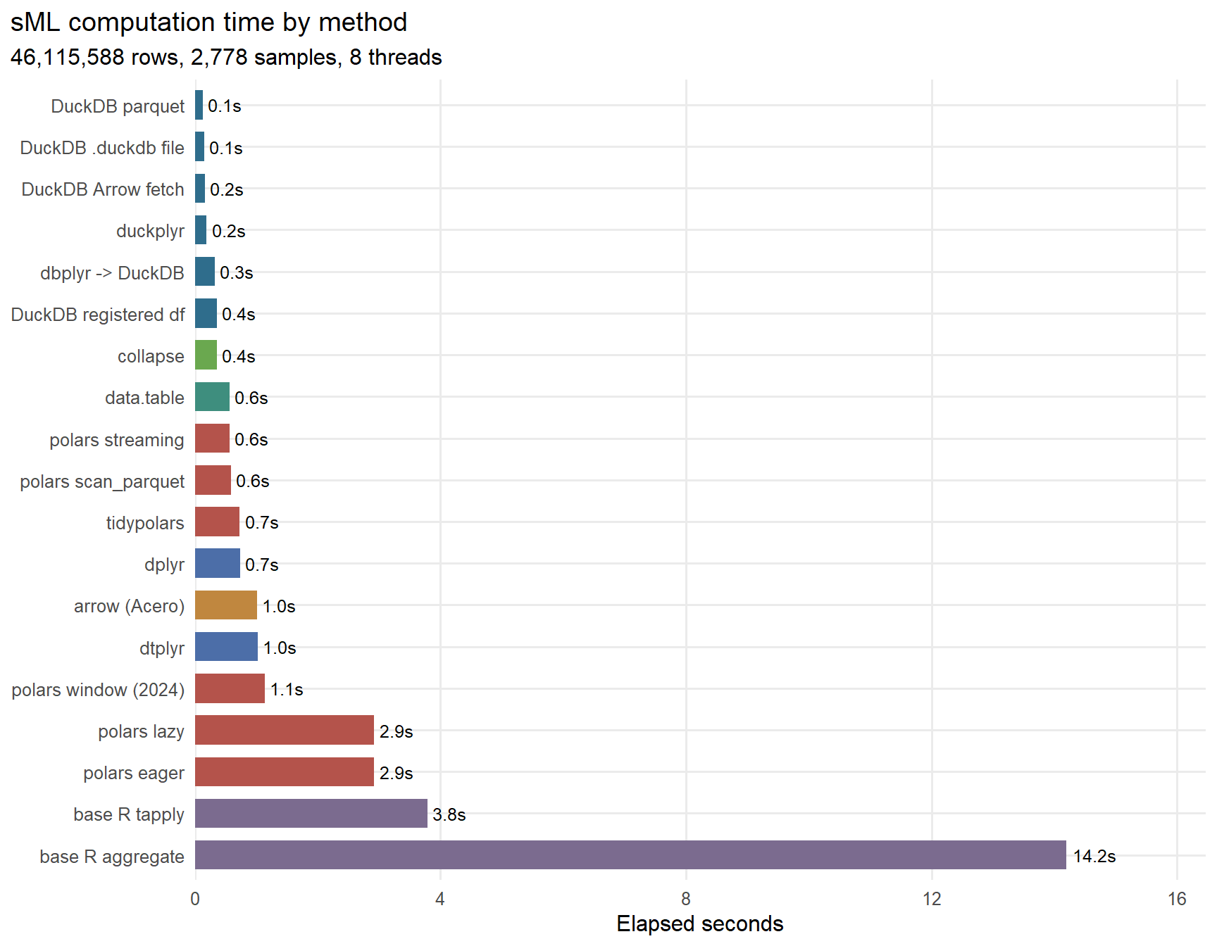

Figure 2: Time to compute sMF for every sample. Bars are colored by tool family; all methods return an identical table.

compute_res |>
  subset(!is.na(delta_gb)) |>
  transform(marginal = pmax(delta_gb, 0)) |>
  (\(x) transform(x, method = factor(method, levels = method[order(x$marginal)])))() |>
  ggplot(aes(marginal, method, fill = family)) +
  geom_col(width = .7) +
  geom_text(aes(label = sprintf("%.2f", marginal)), hjust = -0.15, size = 3.3) +
  scale_fill_manual(values = fam_pal) +
  scale_x_continuous(expand = expansion(mult = c(0, .18))) +
  labs(title = "Marginal peak memory by method",
       subtitle = sprintf("Above a baseline of ~%.1f GB with the data frame loaded",
                          stats::median(compute_res$base_gb, na.rm = TRUE)),
       x = "Peak RSS above baseline (GB)", y = NULL)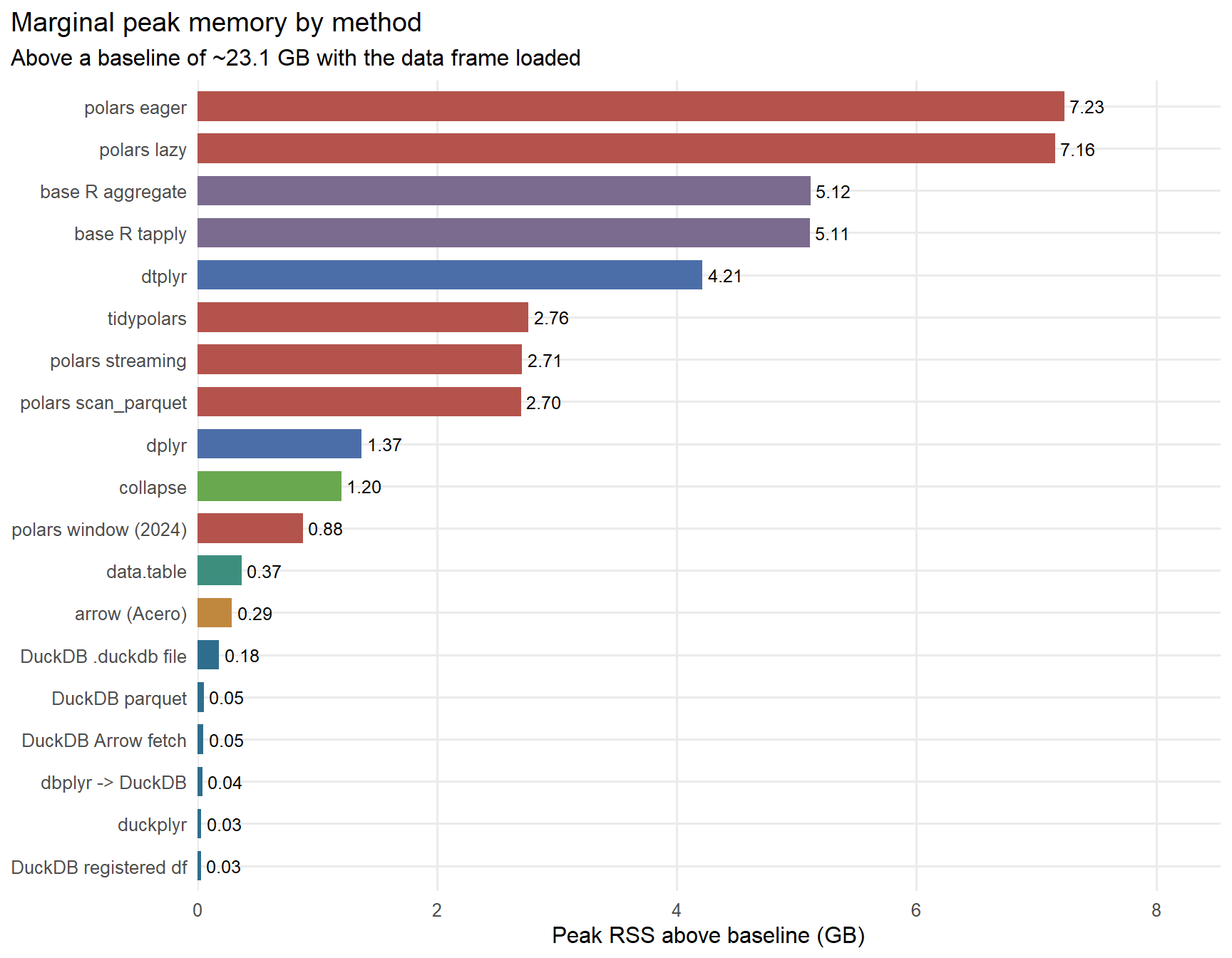

Figure 3: Memory each method needs on top of what the session already holds. The in-memory data frame is loaded throughout, so absolute peak RSS is dominated by that shared baseline; the marginal cost is the honest comparison.

ImportantRead that chart carefully — it understates the file-backed engines

Every method above runs in a session where d, the full in-memory data frame, is already loaded, because the base R and dplyr methods need it. So the absolute peak RSS is roughly the same for all of them and tells you nothing.

The chart therefore plots the marginal cost: how much memory each method adds on top of that shared baseline. But this still flatters the in-memory methods, because they are getting their copy of the data for free — someone already paid for it.

The fair statement is the one the file-backed engines make possible: polars scan_parquet, polars streaming, DuckDB parquet and duckplyr never need d to exist at all. In a session that only ever runs those, the baseline is a few hundred megabytes rather than several gigabytes — the data frame is simply never materialized. That is the difference Section 8 makes concrete by putting DuckDB under a hard memory limit.

compute_res |>
  subset(!is.na(elapsed) & !is.na(peak_gb)) |>
  ggplot(aes(elapsed, peak_gb, color = family, label = method)) +
  geom_point(size = 3.2, alpha = .85) +
  ggrepel::geom_text_repel(size = 3, max.overlaps = 20, seed = 1) +
  scale_color_manual(values = fam_pal) +
  scale_x_log10() +
  labs(title = "The actual trade-off", x = "Elapsed seconds (log scale)",
       y = "Peak RSS (GB)")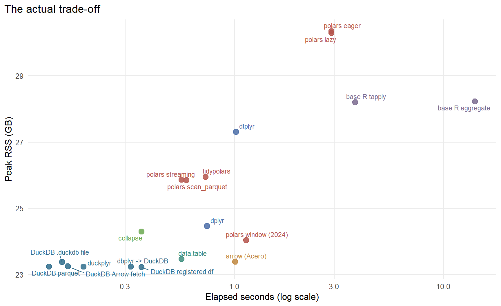

Figure 4: Time against memory. Bottom-left is better. Note the cluster of file-backed engines that are both fast and light.

7.6 How stable are these numbers?

Everything above is a single run, which is honest about cost but says nothing about variance. bench::mark() repeats each expression and reports the distribution — and its check argument gives us the correctness comparison for free if we hand it canon().

mark_res <- bench::mark(
  collapse   = sml_collapse(),
  data.table = sml_datatable(),
  polars     = sml_polars_streaming(),
  duckdb     = sml_duckdb_parquet(),
  check      = function(a, b) isTRUE(all.equal(canon(a), canon(b), tolerance = 1e-8)),
  iterations = 5,
  filter_gc  = FALSE,      # at this size every iteration triggers GC; keep them all
  memory     = FALSE       # mem_alloc cannot see DuckDB/Polars -- see @sec-bench
)

mark_res |>
  dplyr::transmute(
    expression = as.character(expression),
    min        = as.numeric(min),
    median     = as.numeric(median),
    max        = vapply(time, function(t) max(as.numeric(t)), numeric(1)),
    sd         = vapply(time, function(t) stats::sd(as.numeric(t)), numeric(1)),
    n_itr      = n_itr
  ) |>
  kable(digits = 3, caption = "Five iterations each; times in seconds")

Five iterations each; times in seconds

expression	min	median	max	sd	n_itr
collapse	0.341	0.370	0.522	0.075	5
data.table	0.554	0.560	0.565	0.004	5
polars	0.556	0.574	0.576	0.008	5
duckdb	0.128	0.129	0.137	0.004	5

autoplot(mark_res) + labs(title = "Repeated measurements")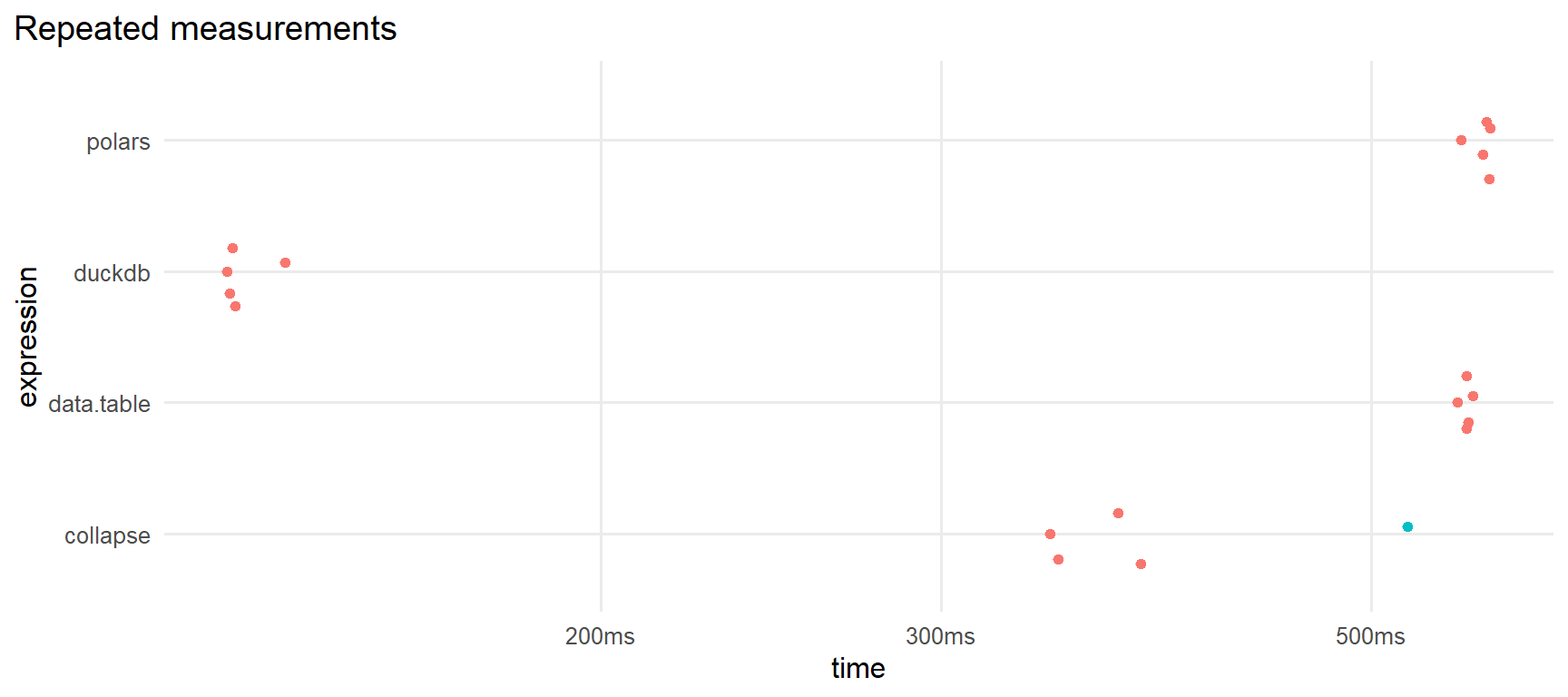

Figure 5: Distribution across five iterations. Wide spread usually means the OS cache or GC is interfering rather than the engine being erratic.

Notememory = FALSE is deliberate

bench::mark()’s mem_alloc column comes from Rprofmem and has exactly the blind spot described in Section 4 — it reports 0B for work done inside DuckDB or Polars. Leaving the column on would produce a table implying those engines are free. Time comes from bench; memory comes from the RSS sampler.

8 Part 4 — Scaling and memory pressure

8.1 Does it get faster with more threads?

thread_grid <- c(1, 2, 4, 8, params$threads) |> unique() |> sort()
sweep_rows <- lapply(thread_grid, function(nthr) {
  duck <- measure({
    cc <- dbConnect(duckdb(), config = list(threads = as.character(nthr)))
    on.exit(dbDisconnect(cc, shutdown = TRUE), add = TRUE)
    dbGetQuery(cc, duck_sql(sprintf("read_parquet('%s')", PQ)))
  }, sample_mem = FALSE)
  data.table::setDTthreads(nthr)
  dtt <- measure(sml_datatable(), sample_mem = FALSE)
  data.frame(threads = nthr,
             DuckDB = duck$elapsed, data.table = dtt$elapsed)
})
data.table::setDTthreads(params$threads)
sweep <- do.call(rbind, sweep_rows)
kable(sweep, digits = 2, caption = "Scaling with thread count (seconds)")

Scaling with thread count (seconds)

threads	DuckDB	data.table
1	0.15	0.48
2	0.12	0.41
4	0.14	0.44
8	0.14	0.54

sweep |>
  tidyr::pivot_longer(-threads, names_to = "engine", values_to = "elapsed") |>
  ggplot(aes(threads, elapsed, color = engine)) +
  geom_line(linewidth = .9) + geom_point(size = 2.6) +
  scale_color_manual(values = c(DuckDB = "#2F6D8C", data.table = "#3E8E7E")) +
  scale_x_continuous(breaks = thread_grid) +
  theme(legend.position = "right") +
  labs(title = "Elapsed time vs thread count", x = "Threads", y = "Seconds")

Figure 6: Thread scaling. Perfect scaling would be a straight line to the bottom-right on these axes; real engines flatten out as coordination and I/O start to dominate.

8.2 Working under a hard memory limit

This is the property that actually distinguishes DuckDB and Polars from every in-memory method: they will complete a query that does not fit in RAM, by spilling to disk. We can force it with an artificially tight budget.

The sMF query is a streaming aggregation — it never needs much working memory, so it is a poor test. Instead we force something genuinely memory-hungry: a full sort of all 46 million rows, written back out to Parquet. Sorting cannot emit its first row until it has seen the last one.

sort_out <- tempfile(fileext = ".parquet")
mem_limits <- c("1GB", "4GB", "24GB")

lim_rows <- lapply(mem_limits, function(lim) {
  tdir <- file.path(tempdir(), paste0("duckspill_", gsub("[^A-Za-z0-9]", "", lim)))
  dir.create(tdir, showWarnings = FALSE)
  cc <- dbConnect(duckdb(), config = list(
    threads        = as.character(params$threads),
    memory_limit   = lim,
    temp_directory = gsub("\\\\", "/", tdir)))
  on.exit({ dbDisconnect(cc, shutdown = TRUE); unlink(tdir, recursive = TRUE) }, add = TRUE)

  unlink(sort_out)
  m <- measure(dbExecute(cc, sprintf(
        "COPY (SELECT * FROM read_parquet('%s') ORDER BY VAF, position)
         TO '%s' (FORMAT PARQUET)", PQ, gsub("\\\\", "/", sort_out))),
       sample_mem = TRUE)
  data.frame(memory_limit = lim, elapsed = m$elapsed,
             marginal_gb = m$delta_gb, peak_gb = m$peak_gb)
})
unlink(sort_out)

do.call(rbind, lim_rows) |>
  kable(digits = 2, caption = "A full 46M-row sort under different DuckDB memory limits",
        col.names = c("memory_limit", "Elapsed (s)", "Memory above baseline (GB)",
                      "Peak RSS (GB)"))

A full 46M-row sort under different DuckDB memory limits

memory_limit	Elapsed (s)	Memory above baseline (GB)	Peak RSS (GB)
1GB	2.78	8.63	31.92
4GB	2.78	8.40	31.74
24GB	2.81	8.39	31.70

ImportantWhat that table actually shows — and what it does not

Two things are worth taking from it, and one common claim is not supported.

The query completes at every limit, including one far below the size of the data. DuckDB sorted 46 million rows with its budget set to 1 GB. No in-memory method in this document can do that; base R would have to hold the whole table plus a sorted copy.

But memory_limit did not meaningfully change either runtime or process memory here. That is not a bug. DuckDB’s limit governs its buffer manager; the Parquet reader’s decompression buffers, the writer’s row-group buffers, query results and everything R itself holds all live outside it. Process RSS therefore sits well above the nominal limit no matter what you set, and our sampler correctly reports that. Treat memory_limit as a guard against runaway intermediate state, not as a hard cap on the process. DuckDB’s own guidance is 1–4 GB of limit per thread.

A caveat on honesty: I could not get this query to leave measurable evidence of spilling. duckdb_memory() reports current state, and DuckDB deletes its temp files as soon as the query finishes, so a post-hoc reading is always zero — whether it spilled or not. Measuring spill properly means sampling the temp directory during execution, the same way we sample RSS. Rather than show a table of zeros and imply “no spilling occurred”, the honest statement is: the query completed comfortably under a 1 GB budget, and I did not prove how it did so.

8.3 Scaling with data size

fracs <- c(0.05, 0.15, 0.35, 0.65, 1.0)
tmp_pq <- tempfile(fileext = ".parquet")
curve_rows <- lapply(fracs, function(f) {
  cc <- new_con(); on.exit(dbDisconnect(cc, shutdown = TRUE), add = TRUE)
  n <- round(shape$rows * f)
  dbExecute(cc, sprintf("COPY (SELECT * FROM read_parquet('%s') LIMIT %d) TO '%s'
                         (FORMAT PARQUET, COMPRESSION ZSTD)", PQ, n, tmp_pq))
  a <- measure(dbGetQuery(cc, duck_sql(sprintf("read_parquet('%s')", tmp_pq))), sample_mem = FALSE)
  b <- measure(polars_pipeline(pl$scan_parquet(tmp_pq))$collect(engine = "streaming"),
               sample_mem = FALSE)
  dd <- as.data.frame(arrow::read_parquet(tmp_pq))
  cl <- fmin(dd$cluster_id, g = dd$samplename, TRA = "replace")
  cc2 <- measure({
    n1 <- fnobs(dd$cluster_id, g = dd$samplename)
    n2 <- fsum(dd$cluster_id == cl, g = dd$samplename)
    data.frame(n1, n2)
  }, sample_mem = FALSE)
  rm(dd); gc(FALSE)
  data.frame(rows = n, DuckDB = a$elapsed, polars = b$elapsed, collapse = cc2$elapsed)
})
unlink(tmp_pq)
curve <- do.call(rbind, curve_rows)
kable(curve, digits = 2, caption = "Elapsed seconds vs row count")

Elapsed seconds vs row count

rows	DuckDB	polars	collapse
2305779	0.02	0.03	0.00
6917338	0.03	0.07	0.04
16140456	0.05	0.19	0.07
29975132	0.07	0.36	0.18
46115588	0.13	0.54	0.25

curve |>
  tidyr::pivot_longer(-rows, names_to = "engine", values_to = "elapsed") |>
  ggplot(aes(rows, elapsed, color = engine)) +
  geom_line(linewidth = .9) + geom_point(size = 2.4) +
  scale_color_manual(values = c(DuckDB = "#2F6D8C", polars = "#B4534B", collapse = "#6AA84F")) +
  scale_x_continuous(labels = scales::label_number(scale_cut = scales::cut_short_scale())) +
  theme(legend.position = "right") +
  labs(title = "Scaling with row count", x = "Rows", y = "Seconds")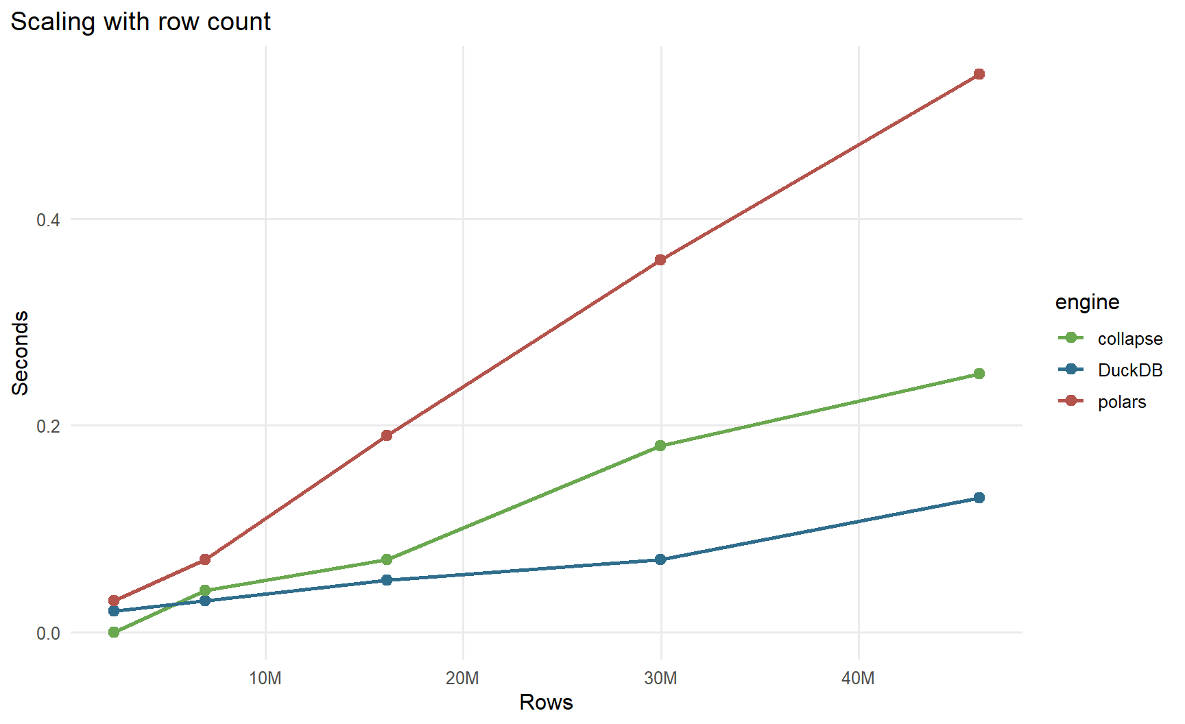

Figure 7: How each engine scales with input size. Straight lines on linear axes indicate the expected O(n) behavior; the intercept is fixed startup cost.

8.4 Larger-than-memory output with sink_parquet()

Every method so far returns a small table. When the output is also large, pulling it into R defeats the purpose. Polars can stream a query straight to a new Parquet file without materializing it:

sink_out <- tempfile(fileext = ".parquet")
m_sink <- measure(
  pl$scan_parquet(PQ)$
    filter(pl$col("cluster_id") == 0L)$
    select("samplename", "chromosome", "position", "VAF")$
    sink_parquet(sink_out),
  sample_mem = TRUE)

cat(sprintf("streamed %.2f GB -> %s in %.1fs, peak RSS %.2f GB\n",
            file.info(sink_out)$size/GB, basename(sink_out), m_sink$elapsed, m_sink$peak_gb))

streamed 0.51 GB -> file9b2c11be99.parquet in 0.4s, peak RSS 24.29 GB

unlink(sink_out)

DuckDB’s equivalent is COPY (...) TO 'out.parquet' (FORMAT PARQUET, COMPRESSION ZSTD), which likewise never routes the data through R.

9 Part 5 — Leaving R

Quarto runs more than R. When a step genuinely does not belong in R — a tight loop, a library that only exists in Python, a numerical kernel — you can drop into another language in the same document and pass data across.

9.1 Python

The R and Python bindings for Polars and DuckDB wrap the same engines, so this is not really a language comparison: it is a measurement of binding overhead and of how each ecosystem hands data back.

WarningWhy these chunks run in a subprocess, not reticulate

The obvious approach is reticulate, which runs Python inside the R process and lets you write r.PQ and py$result. It does not work in this document, and the reason is worth knowing:

library(arrow)                      # R's arrow: loads Arrow C++ DLLs into the process
reticulate::py_run_string("import pyarrow")
#> ImportError: DLL load failed while importing lib:
#>   The specified procedure could not be found.

R’s arrow package and Python’s pyarrow each bundle their own build of the Arrow C++ libraries. Load both into one process on Windows and the dynamic linker resolves pyarrow’s extension against R’s already-loaded DLLs, which export different symbols. polars and duckdb import fine; pyarrow is the casualty. (Verified on this machine: with R arrow unloaded, all three import cleanly.)

Running Python as a separate process sidesteps the whole class of problem, and costs only that data must cross as files rather than as in-memory objects. For a benchmark that is no loss at all — the data is already a file.

NoteCreating the Python environment

The chunks below expect a virtual environment in .venv/ next to this document. With uv (fast, and it will fetch Python itself):

uv venv .venv --python 3.13
uv pip install --python .venv/Scripts/python.exe polars duckdb pyarrow pandas

or with stock Python:

python -m venv .venv
.venv/Scripts/pip install polars duckdb pyarrow pandas

If .venv is absent the Python chunks are skipped and the rest of the document still renders — see the py_ok guard below.

We pass parameters out as JSON and read results back the same way.

py_cfg <- "py_config.json"
jsonlite::write_json(list(pq = normalizePath(PQ, winslash = "/"),
                          threads = params$threads,
                          out = "py_results.json"),
                     py_cfg, auto_unbox = TRUE)

py_exe <- if (file.exists(".venv/Scripts/python.exe")) ".venv/Scripts/python.exe" else
          if (file.exists(".venv/bin/python"))         ".venv/bin/python"        else "python"
py_ok <- nzchar(Sys.which(py_exe)) || file.exists(py_exe)
cat("python:", py_exe, if (py_ok) "(found)" else "(NOT FOUND -- chunk will be skipped)", "\n")

python: .venv/Scripts/python.exe (found) 

import json, time
import polars as pl, duckdb, pyarrow

cfg     = json.load(open("py_config.json"))
PQ      = cfg["pq"]
THREADS = int(cfg["threads"])
print(f"polars {pl.__version__} | duckdb {duckdb.__version__} | pyarrow {pyarrow.__version__}")

# --- Polars, streaming engine -------------------------------------------------
q = (pl.scan_parquet(PQ)
       .group_by("samplename")
       .agg(pl.len().alias("n_snvs"),
            (pl.col("cluster_id") == pl.col("cluster_id").min()).sum().alias("n_clonal"))
       .with_columns((pl.col("n_snvs") - pl.col("n_clonal")).alias("n_subclonal"))
       .with_columns((pl.col("n_subclonal") / pl.col("n_snvs")).alias("sMF")))
t0 = time.perf_counter(); out_pl = q.collect(engine="streaming"); t_pl = time.perf_counter() - t0

# --- DuckDB, results straight to Arrow ----------------------------------------
con = duckdb.connect(config={"threads": THREADS})
sql = f"""
SELECT samplename, COUNT(*) AS n_snvs,
       COUNT(*) FILTER (cluster_id = mn) AS n_clonal,
       COUNT(*) - COUNT(*) FILTER (cluster_id = mn) AS n_subclonal,
       (COUNT(*) - COUNT(*) FILTER (cluster_id = mn))::DOUBLE / COUNT(*) AS sMF
FROM (SELECT samplename, cluster_id,
             MIN(cluster_id) OVER (PARTITION BY samplename) mn
      FROM read_parquet('{PQ}'))
GROUP BY ALL"""
# NB: .arrow() hands back a lazy RecordBatchReader, so timing it alone would
# measure nothing at all -- the lazy trap from @sec-bench, in Python. read_all()
# forces the query to actually run.
t0 = time.perf_counter()
out_db = con.sql(sql).arrow().read_all()
t_db = time.perf_counter() - t0

print(f"python polars (streaming): {t_pl:6.2f}s  -> {out_pl.height} rows")
print(f"python duckdb  (-> arrow): {t_db:6.2f}s  -> {out_db.num_rows} rows")

json.dump({"python polars (streaming)": t_pl,
           "python duckdb (-> arrow)":  t_db,
           "rows": out_pl.height,
           "versions": {"polars": pl.__version__, "duckdb": duckdb.__version__}},
          open(cfg["out"], "w"), indent = 2)

polars 1.43.0 | duckdb 1.5.5 | pyarrow 25.0.0
python polars (streaming):   0.46s  -> 2778 rows
python duckdb  (-> arrow):   0.14s  -> 2778 rows

if (file.exists("py_results.json")) {
  pyr <- jsonlite::read_json("py_results.json", simplifyVector = TRUE)
  r_side <- compute_res[compute_res$method %in%
                        c("polars streaming", "DuckDB parquet"), c("method", "elapsed")]
  rbind(
    data.frame(engine = names(pyr)[1:2], elapsed = unlist(pyr[1:2]), language = "Python"),
    data.frame(engine = r_side$method,   elapsed = r_side$elapsed,   language = "R")
  ) |> kable(digits = 2, row.names = FALSE,
             caption = "Same engines, two languages. Differences here are binding overhead, not engine speed.")
  } else cat("Python chunk did not produce results.\n")

Same engines, two languages. Differences here are binding overhead, not engine speed.

engine	elapsed	language
python polars (streaming)	0.46	Python
python duckdb (-> arrow)	0.14	Python
polars streaming	0.56	R
DuckDB parquet	0.13	R

TipMoving data between languages

Passing a file path across the boundary costs nothing; passing a table costs a full copy and a serialization. The rule for polyglot pipelines is the same as for the engines themselves: move the computation to the data, not the data to the computation. Write Parquet on one side and scan it on the other — both languages read it natively and neither has to materialize it.

9.2 C++ via Rcpp

For this task a hand-written C++ kernel is genuinely competitive: a single hash-map pass computes the grouped minimum and both counts. This is what collapse is doing internally, and what you would write if you needed something collapse does not provide.

Rcpp::cppFunction('
DataFrame sml_cpp(CharacterVector sample, IntegerVector cluster) {
  int n = sample.size();
  std::unordered_map<std::string,int> idx;
  std::vector<std::string> names;
  std::vector<int> mn, tot;
  // pass 1: grouped minimum and row counts
  for (int i = 0; i < n; i++) {
    std::string s = as<std::string>(sample[i]);
    auto it = idx.find(s);
    int j;
    if (it == idx.end()) {
      j = names.size(); idx[s] = j;
      names.push_back(s); mn.push_back(cluster[i]); tot.push_back(0);
    } else j = it->second;
    if (cluster[i] < mn[j]) mn[j] = cluster[i];
    tot[j]++;
  }
  // pass 2: count rows sitting in each group\'s minimum cluster
  std::vector<int> clonal(names.size(), 0);
  for (int i = 0; i < n; i++) {
    int j = idx[as<std::string>(sample[i])];
    if (cluster[i] == mn[j]) clonal[j]++;
  }
  int g = names.size();
  NumericVector sub(g), sml(g);
  for (int j = 0; j < g; j++) { sub[j] = tot[j] - clonal[j]; sml[j] = sub[j] / (double)tot[j]; }
  return DataFrame::create(_["samplename"] = names, _["n_snvs"] = tot,
                           _["n_clonal"] = clonal, _["n_subclonal"] = sub,
                           _["sMF"] = sml, _["stringsAsFactors"] = false);
}',
includes = c("#include <unordered_map>", "#include <string>", "#include <vector>"))

cpp_res <- run_suite(list(
  bench_method("C++ (Rcpp, 1 thread)", "other",
               function() sml_cpp(d$samplename, d$cluster_id), "two-pass hash map"),
  bench_method("collapse", "collapse", sml_collapse, "for reference")
), sample_mem = TRUE)

cpp_res |> subset(select = c(method, note, elapsed, peak_gb, correct)) |>
  kable(digits = 2, caption = "A hand-written kernel against a tuned library",
        col.names = c("Method", "Note", "Elapsed (s)", "Peak RSS (GB)", "Correct"))

A hand-written kernel against a tuned library

Method	Note	Elapsed (s)	Peak RSS (GB)	Correct
C++ (Rcpp, 1 thread)	two-pass hash map	3.23	23.28	reference
collapse	for reference	0.34	24.48	match

ImportantThe hand-written kernel loses, and that is the lesson

Read that table again: the C++ is roughly an order of magnitude slower than the three-line collapse call it was supposed to beat.

The algorithm is fine — one hash-map pass, no wasted work. The problem is this line, executed 92 million times:

std::string s = as<std::string>(sample[i]);

Every row constructs a fresh std::string, copying the characters out of R’s internal string representation, just to use it as a hash key and throw it away. R already interns every string in a global cache, so each unique sample name exists exactly once in memory and collapse can hash the pointer rather than the bytes. The C++ version does an enormous amount of allocation to rediscover something R already knew.

You can fix it — hash the SEXP pointers from STRING_ELT() directly, or factor the column once in R and pass integers to C++. Both work. Both also make the code longer and more dependent on R’s internals, which is precisely the point:

“Rewrite it in C++” is not a performance strategy. A mature library encodes years of exactly this kind of knowledge about where the real costs are. Hand-written code beats it only when you know something about your problem that the library cannot — and on a generic grouped aggregation, you don’t. Reach for collapse first; reach for C++ when you have a computation no library expresses at all, and budget for learning where its sharp edges are.

9.3 Julia

Julia is a strong fit for this class of problem — a JIT-compiled numerical language where a hand-written loop runs at C speed without leaving the interactive session. JuliaCall bridges it to R, and Quarto supports native {julia} chunks.

No Julia toolchain is installed on the machine that rendered this document, so the block below is shown but not executed. To make it live:

1. Install Julia with juliaup — winget install julia -s msstore on Windows, or curl -fsSL https://install.julialang.org | sh elsewhere.
2. using Pkg; Pkg.add(["DataFrames", "Parquet2", "DuckDB", "Chain"])
3. install.packages("JuliaCall") — knitr’s julia engine needs it, and will fail to register the engine without it even for a chunk marked eval: false. That is why this is a plain fenced block rather than an executable chunk.
4. Change the fence below from ```julia to ```{julia}.

using Parquet2, DataFrames, Chain

df = DataFrame(Parquet2.Dataset("fake_pcawg_all.parquet"); copycols = false)

result = @chain df begin
    groupby(:samplename)
    combine(
        nrow => :n_snvs,
        [:cluster_id] => (c -> sum(c .== minimum(c))) => :n_clonal,
    )
    transform(
        [:n_snvs, :n_clonal] => ((a, b) -> a .- b) => :n_subclonal,
    )
    transform(
        [:n_snvs, :n_clonal] => ((a, b) -> (a .- b) ./ a) => :sMF,
    )
end

From R, the equivalent through JuliaCall:

library(JuliaCall)
julia_setup()
julia_library("DataFrames"); julia_library("Parquet2")
julia_assign("path", PQ)
julia_eval('
  using Parquet2, DataFrames
  df = DataFrame(Parquet2.Dataset(path); copycols=false)
  combine(groupby(df, :samplename), nrow => :n_snvs)
')

NoteThe honest assessment

For this task Julia has little to offer over DuckDB or Polars — the work is a grouped aggregation, which is exactly what those engines are built for, and Parquet2.jl is less mature than Arrow’s reader. Julia earns its place when the inner computation is custom numerics that no query engine expresses: simulation, optimization, differential equations. Reaching for it to do a GROUP BY means paying the compilation latency and the interop cost for nothing.

9.4 Rust

There is a certain circularity in benchmarking Rust here: Polars is Rust, and the polars calls throughout this document already run compiled Rust. Arrow’s core and much of DuckDB’s ecosystem tooling are similar stories.

So the interesting question is not “is Rust fast” but “what if I need a kernel Polars does not have?” The answer is extendr, which is to Rust what Rcpp is to C++. rextendr provides a rust_function() helper and a knitr engine, so Rust can live in a chunk.

Not evaluated — no Rust toolchain here. Install rustup and install.packages("rextendr"), then set eval: true.

rextendr::rust_function('
  fn sml_rust(cluster: Vec<i32>, group: Vec<i32>, n_groups: usize) -> Vec<f64> {
      let mut mn  = vec![i32::MAX; n_groups];
      let mut tot = vec![0usize;  n_groups];
      for (c, g) in cluster.iter().zip(group.iter()) {
          let g = *g as usize;
          if *c < mn[g] { mn[g] = *c; }
          tot[g] += 1;
      }
      let mut clonal = vec![0usize; n_groups];
      for (c, g) in cluster.iter().zip(group.iter()) {
          let g = *g as usize;
          if *c == mn[g] { clonal[g] += 1; }
      }
      (0..n_groups).map(|j| (tot[j] - clonal[j]) as f64 / tot[j] as f64).collect()
  }
')

The realistic reason to reach for extendr is not speed — it is that you want memory safety and Rust’s ecosystem (including polars-rs itself) inside an R package, without hand-managing the lifetimes that make the Rcpp version above something you have to review carefully.

10 Part 6 — Choosing

10.1 What the numbers say

compute_res |>
  subset(!is.na(elapsed)) |>
  (\(x) x[order(x$family, x$elapsed), ])() |>
  (\(x) x[!duplicated(x$family), ])() |>
  transform(relative = round(elapsed / min(elapsed, na.rm = TRUE), 1)) |>
  subset(select = c(family, method, elapsed, relative, peak_gb)) |>
  kable(digits = 2, caption = "Fastest representative of each tool family",
        col.names = c("Family", "Best method", "Elapsed (s)", "x slowest-in-class", "Peak RSS (GB)"))

Table 3: Fastest representative of each tool family

	Family	Best method	Elapsed (s)	x slowest-in-class	Peak RSS (GB)
7	arrow	arrow (Acero)	1.01	7.8	23.38
2	base R	base R tapply	3.79	29.2	28.20
3	collapse	collapse	0.36	2.8	24.29
6	data.table	data.table	0.56	4.3	23.46
14	DuckDB	DuckDB parquet	0.13	1.0	23.23
11	polars	polars streaming	0.56	4.3	25.86
4	tidyverse	dplyr	0.74	5.7	24.46

10.2 A decision guide

flowchart TD
    A[How big is the data?] -->|Fits in RAM<br/>with room to spare| B[Do you already know<br/>data.table or dplyr?]
    A -->|Larger than RAM,<br/>or close to it| C[Is your team<br/>comfortable with SQL?]
    B -->|dplyr, want it faster<br/>with zero rewriting| D[duckplyr]
    B -->|data.table| E[data.table<br/>already excellent]
    B -->|Want maximum speed<br/>in base R idioms| F[collapse]
    C -->|Yes| G[DuckDB + SQL]
    C -->|No, prefer dplyr| H[duckplyr or dbplyr]
    C -->|No, prefer a<br/>DataFrame API| I[Polars<br/>scan + streaming]
    G --> J{Query the same data<br/>many times?}
    J -->|Yes| K[Import to .duckdb]
    J -->|No, or shared<br/>with others| L[Query Parquet directly]

Figure 8: Choosing a tool. The first question is not about speed.

10.3 Recommendations

Change your storage format before you change your library. Going from TSV to Parquet costs one line and buys most of the benefit on offer. Almost nothing else in this document has that ratio.

If your data fits in memory and you already use data.table, stop here. data.table remains superb at this and no rewrite will pay for itself.

If you use dplyr and want it faster without rewriting, use duckplyr. That is its entire premise and it now delivers. Set prudence = "stingy" while developing so fallbacks surface as errors rather than as mysterious slowness.

If the data does not fit in memory, the choice is DuckDB or Polars, and it is mostly about which interface your group will maintain. DuckDB if SQL is a shared language on your team and you want the mature out-of-core story. Polars if you prefer a DataFrame API and are willing to track a faster-moving library. Both read Parquet directly and both are built to work out-of-core — Section 8 sorts all 46 million rows with DuckDB’s budget set to 1 GB — which is simply not a thing base R can do.

Reach for collapse more than you probably do. It is the best speed-per-unit-of- rewriting in R: base R data structures, base-R-shaped functions, C-level speed.

Do not assume dropping to C++ will help. The hand-written kernel in Section 9 came out roughly ten times slower than collapse, because a tuned library already knows where the costs are and a first draft does not. Leave R for a compiled language when you need a computation no library expresses — not for a grouped aggregation.

10.4 Gotchas worth writing down

Trap	Symptom	Fix
profmem on DuckDB/Polars	Engine “uses no memory”	Sample process RSS (Section 4)
pl$DataFrame(df)	Missing-column errors, or a wrong answer	as_polars_df(df)
$collect(streaming = TRUE)	`...` must be empty	$collect(engine = "streaming")
pl$col(c("a","b"))	Invalid input error	pl$col(!!!c("a","b"))
POLARS_MAX_THREADS set late	Thread cap ignored	Set it before library(polars)
Nested aggregate in dbplyr	aggregate function calls cannot be nested	Grouped mutate() then summarize()
Silent duckplyr fallback	Unexpectedly slow	fallback_sitrep(), prudence = "stingy"
Timing a lazy pipeline	Impossibly fast	End in collect()
Timing vroom()	Impossibly fast — it only built an index	altrep = FALSE, or touch every column
Python duckdb.sql(q).arrow()	Returns a lazy RecordBatchReader	.arrow().read_all()
R arrow + pyarrow in one process	DLL load failed while importing lib	Run Python as a subprocess
duckdb_memory() after a query	Spill always reads 0 — temp files already deleted	Sample during execution
“Rewrite the hot loop in C++”	First draft can be slower than the library	Profile before assuming
Cold vs warm page cache	Second engine always wins	Warm the file first, and say so
Reporting user time	Parallel engines look slow	Report elapsed
read.table() without header	Columns named V1…Vn	header = TRUE

11 Conclusion

We implemented one grouped aggregation about twenty ways across five tool families — running it in R, Python and C++, and sketching it in Julia and Rust — and measured each with a harness that can actually see memory allocated outside R.

The consistent finding is that the largest wins come from not moving data. The methods at the top of Figure 2 are the ones that never materialize 46 million rows in R’s heap: they push the computation down to where the bytes already are — a Parquet file — and return only the 2,778-row answer. Base R’s problem on this task is not that aggregate() is a slow function; it is that everything must become an R object first.

Second: the modern tools have converged on making that possible without asking you to abandon the syntax you know. duckplyr and tidypolars both let you write dplyr and execute on a columnar engine. The 2024 edition of this tutorial treated that as aspirational; it is now simply how you should work.

Finally, measure honestly. The original version of this document reported that DuckDB used a fraction of a gigabyte for a query where the true peak was near ten. The conclusion it drew — use DuckDB — happened to survive the correction, but that was luck. Benchmarks that flatter your preferred tool are worse than no benchmarks, because they are persuasive.

sessioninfo::session_info(pkgs = c("polars", "duckdb", "duckplyr", "arrow",
                                   "data.table", "dplyr", "collapse", "tidypolars"))

─ Session info ───────────────────────────────────────────────────────────────
 setting  value
 version  R version 4.5.1 (2025-06-13 ucrt)
 os       Windows 11 x64 (build 26200)
 system   x86_64, mingw32
 ui       RTerm
 language (EN)
 collate  English_United States.utf8
 ctype    English_United States.utf8
 tz       America/New_York
 date     2026-07-27
 pandoc   3.10 @ C:\\Users\\Matthew\\AppData\\Local\\Temp\\claude\\c--Users-Matthew-Downloads-polars-and-duckdb-tutorial\\d22db368-a447-452b-8a32-854a842eedb3\\scratchpad\\quarto\\bin\\tools/ (via rmarkdown)
 quarto   NA

─ Packages ───────────────────────────────────────────────────────────────────
 package     * version date (UTC) lib source
 arrow       * 25.0.0  2026-07-16 [1] CRAN (R 4.5.3)
 assertthat    0.2.1   2019-03-21 [1] CRAN (R 4.5.3)
 bit           4.6.0   2025-03-06 [1] CRAN (R 4.5.1)
 bit64         4.6.0-1 2025-01-16 [1] CRAN (R 4.5.1)
 cachem        1.1.0   2024-05-16 [1] CRAN (R 4.5.1)
 cli           3.6.5   2025-04-23 [1] CRAN (R 4.5.1)
 collapse    * 2.1.7   2026-05-19 [1] CRAN (R 4.5.3)
 collections   0.3.12  2026-03-22 [1] CRAN (R 4.5.3)
 cpp11         0.5.2   2025-03-03 [1] CRAN (R 4.5.1)
 data.table  * 1.17.8  2025-07-10 [1] CRAN (R 4.5.1)
 DBI         * 1.2.3   2024-06-02 [1] CRAN (R 4.5.1)
 dplyr       * 1.2.0   2026-02-03 [1] CRAN (R 4.5.2)
 duckdb      * 1.5.5   2026-07-25 [1] CRAN (R 4.5.3)
 duckplyr    * 1.2.1   2026-03-10 [1] CRAN (R 4.5.3)
 fastmap       1.2.0   2024-05-15 [1] CRAN (R 4.5.1)
 generics      0.1.4   2025-05-09 [1] CRAN (R 4.5.1)
 glue          1.8.0   2024-09-30 [1] CRAN (R 4.5.2)
 jsonlite      2.0.0   2025-03-27 [1] CRAN (R 4.5.1)
 lifecycle     1.0.5   2026-01-08 [1] CRAN (R 4.5.2)
 magrittr      2.0.4   2025-09-12 [1] CRAN (R 4.5.1)
 memoise       2.0.1   2021-11-26 [1] CRAN (R 4.5.1)
 pillar        1.11.1  2025-09-17 [1] CRAN (R 4.5.1)
 pkgconfig     2.0.3   2019-09-22 [1] CRAN (R 4.5.1)
 polars      * 1.13.0  2026-07-04 [1] https://r-multiverse.r-universe.dev (R 4.5.3)
 purrr         1.2.1   2026-01-09 [1] CRAN (R 4.5.2)
 R6            2.6.1   2025-02-15 [1] CRAN (R 4.5.1)
 Rcpp          1.1.2   2026-07-05 [1] CRAN (R 4.5.3)
 rlang         1.3.0   2026-07-05 [1] CRAN (R 4.5.3)
 S7            0.2.2   2026-04-20 [1] https://r-multiverse.r-universe.dev (R 4.5.3)
 stringi       1.8.7   2025-03-27 [1] CRAN (R 4.5.0)
 stringr       1.6.0   2025-11-04 [1] CRAN (R 4.5.2)
 tibble        3.3.1   2026-01-11 [1] CRAN (R 4.5.2)
 tidypolars  * 0.19.0  2026-07-04 [1] https://r-multiverse.r-universe.dev (R 4.5.3)
 tidyr         1.3.2   2025-12-19 [1] CRAN (R 4.5.2)
 tidyselect    1.2.1   2024-03-11 [1] CRAN (R 4.5.1)
 utf8          1.2.6   2025-06-08 [1] CRAN (R 4.5.1)
 vctrs         0.7.1   2026-01-23 [1] CRAN (R 4.5.2)
 withr         3.0.2   2024-10-28 [1] CRAN (R 4.5.1)

 [1] C:/Users/Matthew/AppData/Local/R/win-library/4.5
 [2] C:/Program Files/R/R-4.5.1/library
 * ── Packages attached to the search path.

──────────────────────────────────────────────────────────────────────────────